Introduction to Clustering

Clustering is a cornerstone technique in unsupervised machine learning, where the goal is to automatically discover natural groupings within data without any predefined labels or categories. Unlike supervised learning—which relies on known outcomes—clustering invites the algorithm to find its own structure within the dataset, based purely on similarities among data points. This approach is widely used in real-world applications such as customer segmentation for personalized marketing, anomaly detection in cybersecurity, and biological data analysis to identify gene or protein families. In the context of this project, clustering offers a powerful, unbiased way to explore and categorize food items based entirely on their nutritional profiles, without prior assumptions about how foods should be grouped. By analyzing attributes like calories, sugars, fats, fiber, and protein content, clustering enables the discovery of hidden dietary patterns that may not be immediately obvious through traditional classification. Ultimately, applying clustering to nutrition data helps reveal underlying trends in food composition, consumer preferences, and even potential nutritional gaps—laying the foundation for smarter, more personalized food recommendations.

In this project, three distinct clustering techniques were explored, each offering a unique lens through which to understand the structure of nutritional data:

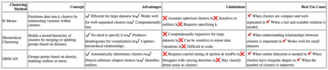
• K-Means Clustering: A popular partition-based method that divides data points into a predefined number of clusters by minimizing the distance between points and their assigned cluster centers. It excels when the data exhibits clear, spherical groupings and provides an efficient, scalable approach to clustering large datasets.
• Hierarchical Clustering: An agglomerative technique that builds a tree-like structure known as a dendrogram, revealing nested relationships between food items. It does not require predefining the number of clusters, making it ideal for uncovering multi-level hierarchies and understanding how closely different items are related at various levels of granularity.
• DBSCAN (Density-Based Spatial Clustering of Applications with Noise): A powerful density-based algorithm that identifies clusters based on areas of high data point density, while simultaneously detecting outliers. Unlike K-Means, DBSCAN can find clusters of arbitrary shapes and is exceptionally robust to noise, making it ideal for complex, non-linear nutritional patterns where traditional partitioning methods might fail.

Each clustering method brings its own strengths and limitations to the table, offering diverse insights into the underlying nutritional patterns:

• K-Means Clustering: Highly efficient and scalable, making it ideal for large datasets. However, it operates best when clusters are spherical and similarly sized, which may not always align with the natural structure of real-world nutritional data.
• Hierarchical Clustering: Provides a detailed, tree-like view of data relationships, capturing multiple layers of similarity between food items. While it excels at revealing complex hierarchies, it can be computationally intensive, particularly for larger datasets.
• DBSCAN: Exceptionally good at detecting clusters of arbitrary shapes and identifying outliers, making it a powerful tool for irregular data landscapes. However, it requires careful tuning of parameters like epsilon and minimum points, which can influence the quality and stability of the resulting clusters.

Understanding Distance Metrics in Clustering

Clustering algorithms rely on distance metrics to measure how similar or different data points are. The choice of metric impacts cluster formation and overall accuracy. Below are common distance measures used in K-Means, Hierarchical Clustering, and DBSCAN.

Common Distance Metrics

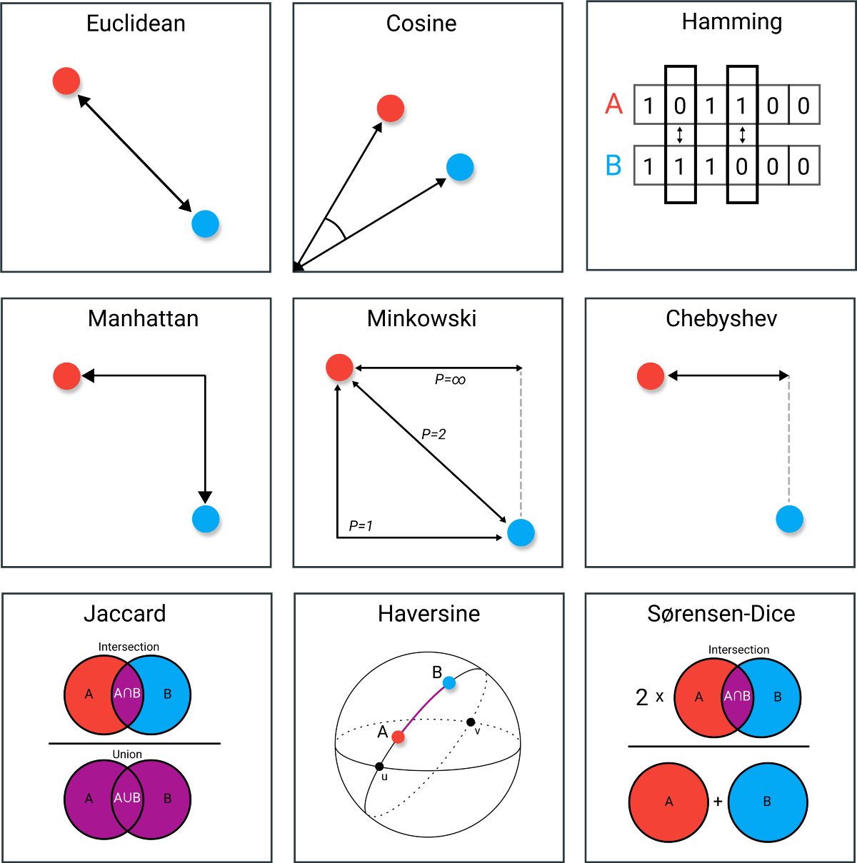
• Euclidean Distance: Often visualized as the straight-line distance between two points in space, Euclidean distance is the most intuitive and widely used metric. In clustering algorithms like K-Means and DBSCAN, it helps in grouping points that are closer together geometrically. It assumes the data lies in a continuous, isotropic space where proximity equates to similarity. However, Euclidean distance may become less effective in very high-dimensional datasets, where the "curse of dimensionality" can distort true similarities.
• Cosine Similarity: Instead of focusing on distance, cosine similarity measures the orientation between two vectors. It calculates the cosine of the angle separating them, making it ideal for comparing text documents or high-dimensional datasets where magnitude differences are less important than directional trends. Used heavily in text clustering and often in hierarchical clustering, this metric shines when the actual values matter less than the overall shape or composition of the vectors.
• Hamming Distance: Specifically tailored for categorical or binary data, Hamming distance counts the number of positions at which corresponding elements differ. It is particularly useful when clustering data like genetic sequences, text encoded as binary, or survey responses. Hamming distance provides a simple yet powerful way to quantify dissimilarity when attributes are not numeric but rather binary outcomes like "yes/no" or "present/absent."
• Manhattan Distance: Also known as "taxicab" distance, Manhattan distance measures the sum of absolute differences across dimensions. This metric mimics how a taxi would navigate a city grid—turning at intersections rather than traveling diagonally. It works well for K-Means clustering when feature scales differ or when the data structure inherently favors stepwise (grid-like) movement rather than straight-line measurements.
• Minkowski Distance: A generalization that encompasses both Euclidean and Manhattan distances. By adjusting the parameter p, Minkowski distance can be tuned to behave like Manhattan (p=1) or Euclidean (p=2). It provides a flexible tool for clustering, allowing researchers to experiment and choose a distance metric that best matches their data’s underlying geometry.
• Chebyshev Distance: Instead of summing or squaring differences, Chebyshev distance simply finds the largest absolute difference along any coordinate dimension. It's particularly useful in environments where one dominant feature can determine cluster membership—such as maximum deviation in a critical nutrient or ingredient that sharply separates different types of food products.
• Jaccard Similarity: A set-based metric that measures the proportion of shared elements between two sets. Jaccard is excellent for clustering binary, categorical, or text data where overlap matters more than absolute counts. It’s commonly used in applications like document clustering, social network analysis, and biological data comparisons where "intersection over union" provides meaningful similarity estimates.
• Haversine Distance: Specially designed for measuring the shortest distance between two points on a sphere, Haversine distance is indispensable in geo-spatial clustering—such as mapping food consumption patterns across different regions or studying regional dietary variations. It accounts for the Earth's curvature, making it ideal for clustering based on real-world geographic coordinates.
• Sørensen-Dice Coefficient: Similar in spirit to Jaccard similarity but more sensitive to common elements. The Sørensen-Dice coefficient doubles the weight of shared features, making it especially suited for biological clustering tasks, string matching, and medical data analysis where even slight overlaps carry important meaning.

Impact of Distance Metrics on Clustering

Different clustering algorithms are tailored to work best with particular distance metrics, and the choice of metric can significantly impact the quality and interpretability of clusters:

• K-Means: Primarily utilizes Euclidean distance to create spherical clusters. As a result, it assumes that all clusters have similar density and size, which can sometimes limit its ability to accurately group irregularly distributed food items or highly skewed nutrient profiles.
• Hierarchical Clustering: Is flexible with distance metrics, allowing practitioners to select cosine similarity, Jaccard distance, or Euclidean distance depending on the nature of the data. This adaptability enables hierarchical models to uncover rich multi-level structures in both numerical and categorical datasets, like layered similarities between processed and natural foods.
• DBSCAN: Typically uses Euclidean distance but is not restricted to it. It can be modified to incorporate custom distance metrics like Haversine for spatial data or Manhattan for grid-like distributions. Because DBSCAN relies on density estimation rather than shape assumptions, choosing the right distance metric is crucial to accurately detect organic cluster boundaries and outliers.

Choosing the right distance metric is crucial for obtaining meaningful clusters. For datasets with high-dimensional features, cosine similarity is often more effective, while for continuous numerical data, Euclidean distance remains a standard choice.

Clustering Implementation: Dataset Overview

The dataset used for clustering consists of various food items with multiple nutritional attributes, such as macronutrient composition, vitamin content, and caloric density. The goal is to identify natural groupings within the dataset that reflect dietary patterns and food classifications.

Feature Selection

To ensure the clustering algorithms work effectively, only numerical attributes were retained. The following transformations were applied:

• Removal of categorical attributes: Non-numeric data such as food brand names were excluded.
• Selection of key nutritional metrics: Macronutrient composition (carbohydrates, proteins, fats) and energy content were prioritized.

Data Preparation

Before applying clustering algorithms, the dataset underwent rigorous preprocessing. This step is critical to ensure that clustering methods operate efficiently and accurately. The preprocessing steps included:

• Handling Missing Values: Missing numerical values were imputed using the median or mean, ensuring consistency.
• Feature Scaling: StandardScaler was applied to normalize features, preventing attributes with larger ranges from dominating the clustering process.
• Dimensionality Reduction: Principal Component Analysis (PCA) was used to reduce redundant information and optimize computation.

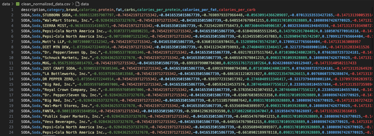
The visualization above shows the dataset after normalization. Scaling ensures that all features contribute equally to distance calculations used in clustering.

Generated Clustering Data

After preprocessing, the dataset was structured in a format suitable for clustering. The processed dataset contains only numerical values for clustering algorithms to analyze effectively.

The table below provides a preview of the cleaned dataset, ready for clustering:

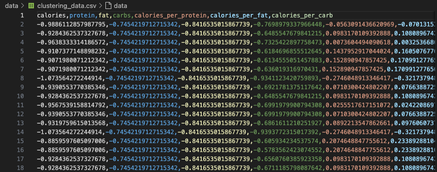
Key transformations applied to this dataset:

• Feature Scaling: Standardized all numerical attributes to have zero mean and unit variance.
• Dimensionality Reduction: Reduced the dataset to key components that explain most of the variance.
• Cluster Compatibility: Removed outliers and ensured that all remaining features were suitable for clustering analysis.

Summary of Data Preparation

The data preprocessing steps were crucial in ensuring high-quality input for clustering. The key takeaways from this process are:

• All categorical variables were removed to ensure clustering algorithms work optimally.
• Missing values were handled efficiently, preventing any data bias.
• Feature scaling ensured that numerical attributes contributed equally to clustering.
• PCA transformation helped reduce dimensionality while retaining the most important information.

With the dataset now optimized for clustering, we proceed to apply the K-Means, Hierarchical, and DBSCAN clustering methods to uncover patterns in food classification.

K-Means Clustering

K-Means is a widely used clustering algorithm that partitions data into a predefined number of clusters (k). It operates iteratively to assign data points to the nearest cluster centroid while updating the centroids until convergence. The objective is to minimize intra-cluster variance, ensuring that data points within the same cluster are as similar as possible.

Determining the Optimal Number of Clusters

Selecting the appropriate number of clusters (k) is crucial for achieving meaningful clustering. A poorly chosen k-value can lead to underfitting (too few clusters) or overfitting (too many clusters). To determine the optimal number of clusters, we used the Silhouette Score, which measures the compactness of clusters and their separation from other clusters. A higher silhouette score indicates well-defined clusters.

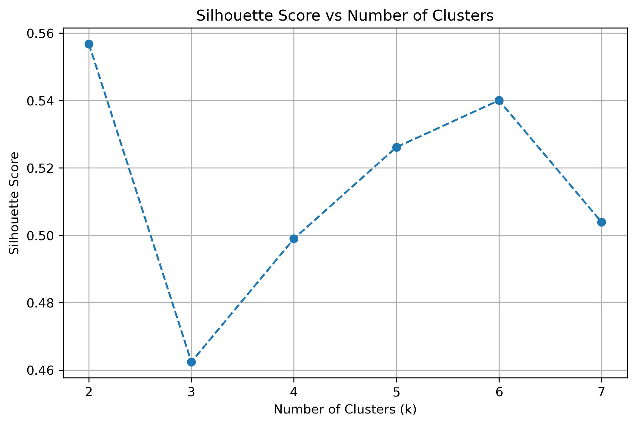
The plot above illustrates how the silhouette score varies across different values of k. The peaks in the graph represent the most suitable choices for k, as they indicate the best balance between cluster compactness and separation. Based on this analysis, the three most effective k-values were selected for clustering.

3D K-Means Clustering Visualization

After determining the optimal k-values, K-Means clustering was applied to the dataset. To better visualize how the clusters are formed, we used Principal Component Analysis (PCA) to reduce the dataset to three principal components (PC1, PC2, PC3), which allowed for a clear 3D representation of the clustering results.

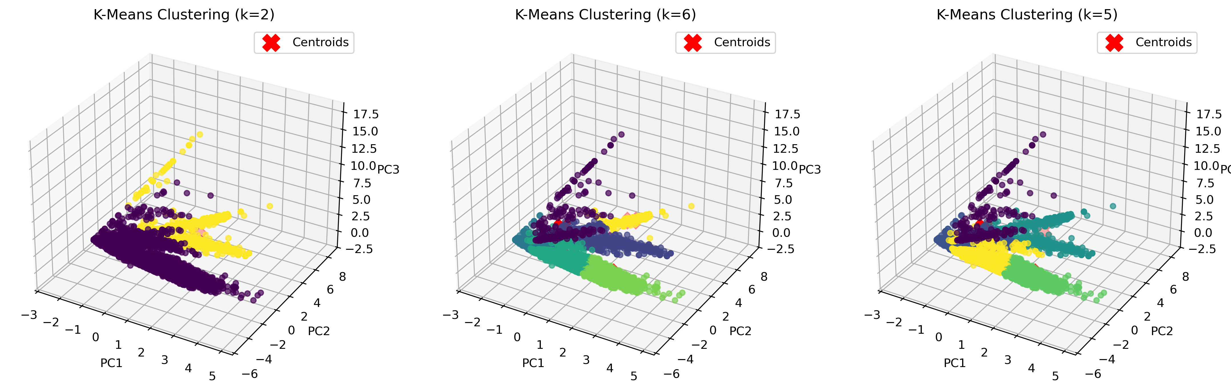
The visualization above represents K-Means clustering for three different values of k. Each color represents a distinct cluster, and the red markers indicate cluster centroids. The plots highlight how increasing k influences cluster separation. Some key observations:

• For k=2, the algorithm splits the data into two large groups, which may be too broad to capture nuanced structures.
• For k=6, the clusters become more refined, but some smaller clusters may not have strong differentiation.
• For k=5, the balance between compactness and meaningful separation appears optimal.

Why These K Values?

The Silhouette Score analysis was instrumental in determining the most suitable k-values. The highest peaks in the silhouette score plot indicate the values of k where clusters are most well-defined and least overlapping.

• k = 2: Simpler division but lacks specificity in distinguishing different groups.
• k = 5: Strikes a balance between cluster cohesion and interpretability.
• k = 6: Offers more refined groupings but may introduce unnecessary complexity.

These selected k-values provided the most stable and interpretable clusters while avoiding over-segmentation of the data.

Observations

The application of K-Means clustering to the dataset led to the following observations:

• K-Means effectively identified meaningful patterns in the dataset, separating different food categories based on nutritional composition.
• The Silhouette Score guided the selection of optimal k-values, ensuring compact and well-separated clusters.
• Some clusters exhibit slight overlaps, indicating that alternative clustering methods like DBSCAN might be more effective in identifying varying densities.

Hierarchical Clustering

Hierarchical Clustering is a bottom-up clustering technique that builds a hierarchy of clusters by progressively merging smaller clusters into larger ones. Unlike K-Means, it does not require a predefined number of clusters. Instead, it generates a tree-like structure called a dendrogram, which visually represents how data points are grouped at various levels of similarity.

Dendrogram Analysis

A dendrogram is a visual representation of the clustering hierarchy. Each point in the tree represents a cluster, and the height at which two clusters merge indicates their similarity. The higher the merge, the greater the difference between clusters.

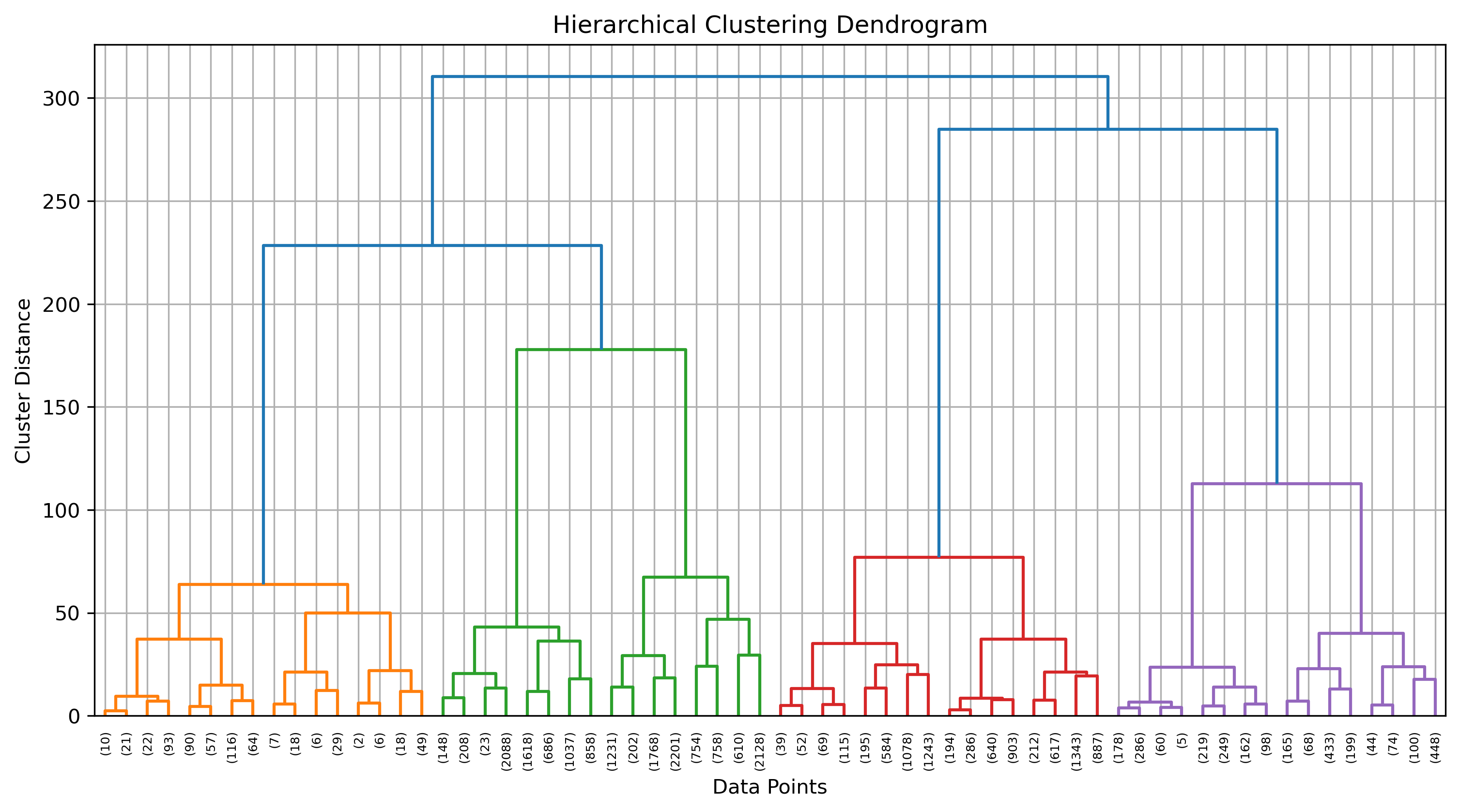
The above dendrogram helps in determining the optimal number of clusters. By cutting the dendrogram at different heights, we can analyze different levels of cluster granularity. This flexibility allows us to explore relationships between food groups without a strict assumption about the number of clusters.

3D Visualization of Hierarchical Clustering

To better understand how hierarchical clustering grouped our dataset, we visualized the clusters using a 3D PCA transformation. This allows us to observe how food items are distributed based on their nutrient compositions.

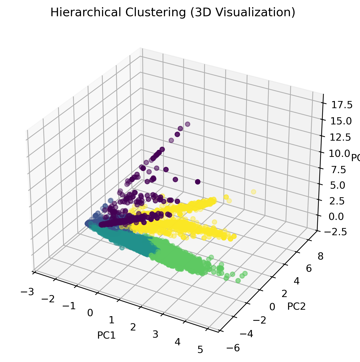
In the visualization above, different colors represent distinct clusters identified by hierarchical clustering. Unlike K-Means, which forces each data point into a cluster, hierarchical clustering preserves the underlying structure and allows us to observe relationships between different groups at varying levels of similarity.

Why Choose Hierarchical Clustering?

Hierarchical Clustering offers several advantages compared to traditional clustering methods like K-Means:

• No need to predefine the number of clusters: Unlike K-Means, which requires choosing k in advance, hierarchical clustering allows us to explore the dataset naturally.
• Provides a complete hierarchy: The dendrogram gives a detailed visualization of how clusters are formed at different levels.
• Works well for small to medium-sized datasets: Since it calculates all pairwise distances, it is computationally expensive for very large datasets but excellent for detailed analysis.
• Identifies nested structures: It is useful when clusters have sub-clusters within them, allowing a more refined categorization.

Limitations of Hierarchical Clustering

Despite its strengths, hierarchical clustering has some limitations:

• Computationally expensive: The algorithm has a complexity of O(n²), making it inefficient for very large datasets.
• Sensitive to noise and outliers: Since it considers all data points in a distance matrix, outliers can distort the clustering structure.
• Inflexibility after clustering: Once the hierarchy is built, it cannot be modified without recalculating the entire dendrogram.

Observations and Key Insights

- Hierarchical clustering successfully captured distinct food groupings based on their nutritional attributes. - The dendrogram provided insights into nested structures, revealing how certain food types share similar characteristics at different hierarchical levels. - This method is particularly useful when we do not know the exact number of clusters in advance, allowing for a more flexible approach to categorizing food items.

DBSCAN Clustering

DBSCAN (Density-Based Spatial Clustering of Applications with Noise) is a density-based clustering algorithm that groups data points based on their proximity to each other. Unlike K-Means or Hierarchical Clustering, DBSCAN does not require specifying the number of clusters beforehand. Instead, it detects dense regions of data and considers low-density points as noise or outliers.

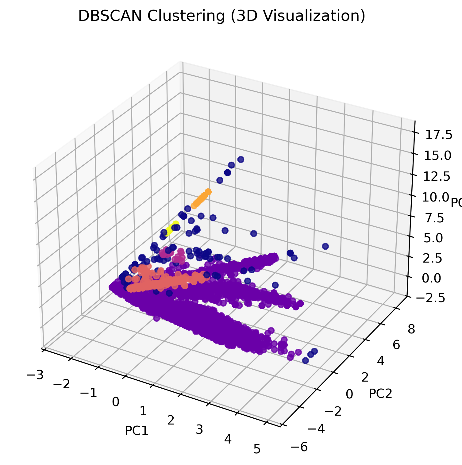
The visualization above illustrates how DBSCAN clusters data in three-dimensional space. Unlike K-Means, which assigns every data point to a cluster, DBSCAN allows certain points to remain unclassified if they are too far from any dense cluster. These unclassified points, often labeled as "outliers," are displayed separately in the visualization.

DBSCAN Algorithm Parameters

DBSCAN operates by defining two critical parameters:

• Epsilon (ε): The maximum distance between two points for them to be considered in the same neighborhood.
• Minimum Points (minPts): The minimum number of points required to form a dense cluster.

If a point has at least minPts neighbors within a radius of ε, it becomes a "core point" and expands a cluster. Points that are within ε distance of a core point but do not have enough neighbors to form their own cluster are considered "border points." Any point that does not fit into these categories is labeled as noise.

Advantages of DBSCAN

• Does not require the number of clusters to be specified, unlike K-Means.
• Can identify clusters of arbitrary shape, which makes it more flexible than K-Means.
• Effectively detects outliers as noise, reducing the impact of anomalies on clustering results.

Limitations of DBSCAN

• Sensitive to parameter selection: The choice of ε and minPts can significantly impact results.
• Not ideal for varying-density clusters: When clusters have different densities, DBSCAN might not perform optimally.
• Computationally expensive for large datasets: DBSCAN has a higher time complexity compared to K-Means.

Comparison of Clustering Performance

The Silhouette Score was used to evaluate and compare the effectiveness of each clustering method. This metric measures how similar each data point is to its assigned cluster compared to other clusters. A higher Silhouette Score indicates better separation between clusters, meaning the clustering method is more effective.

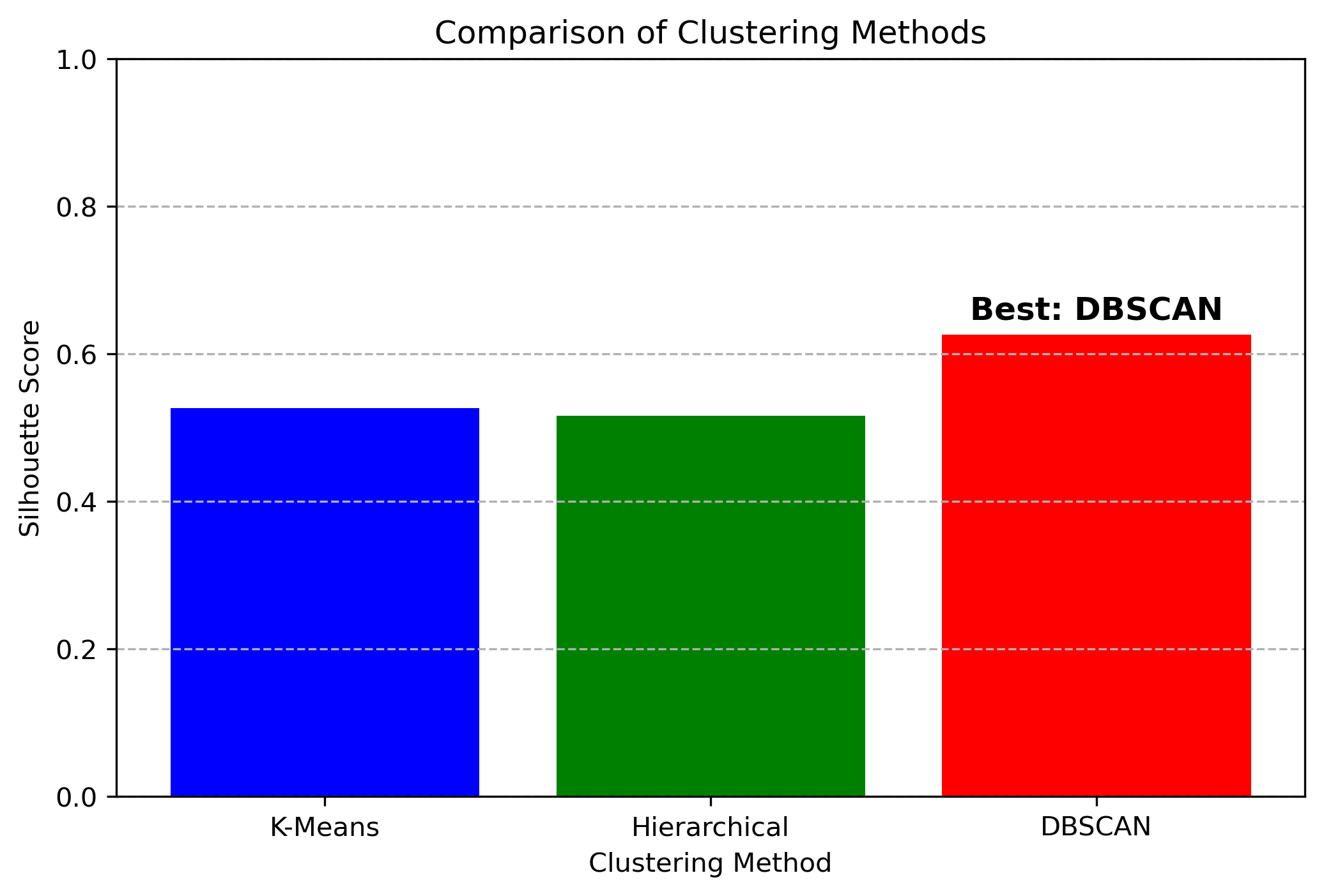
The bar chart above provides a direct comparison of Silhouette Scores across the three clustering methods:

• K-Means (blue bar) achieved a moderate score, indicating that it formed well-defined clusters, but struggled slightly with irregularly shaped or overlapping clusters.
• Hierarchical Clustering (green bar) performed similarly to K-Means, showing strong relationships within clusters but with slightly more flexibility.
• DBSCAN (red bar) achieved the highest Silhouette Score, making it the best-performing method for this dataset.

Comparing Clusters with Original Labels

After clustering, the results were compared to the original labels stored before preprocessing. Here are key observations:

• Some clusters strongly correspond to original food categories (e.g., high-protein foods forming a distinct cluster).
• Other clusters highlight hidden relationships between certain food items that were not evident in the labeled dataset.

Key Observations

• DBSCAN outperformed the other methods, demonstrating its ability to detect clusters of varying shapes and densities while effectively handling noise and outliers.
• K-Means and Hierarchical Clustering produced similar scores, indicating that while both methods structured the data well, they may have struggled with non-spherical clusters or varying densities.
• The high score of DBSCAN suggests that the dataset contains complex cluster structures that do not conform to the strict assumptions made by K-Means and Hierarchical Clustering.

Conclusion

Understanding food composition is crucial for making informed dietary choices. By utilizing clustering techniques, we can uncover hidden patterns within food data that provide valuable insights into nutritional similarities and differences. These insights can help in designing healthier meal plans, improving food recommendations, and identifying potentially misleading food classifications.

The study of food clustering showcases how different items relate to one another based on their macronutrient distribution. Traditional methods of categorizing food by name or brand often fail to reflect their true nutritional composition. However, through clustering, we can identify groups of foods that share similar characteristics, regardless of how they are marketed or labeled.

Moreover, this approach enables better consumer awareness. For example, individuals looking to reduce sugar intake can use these clusters to find alternatives that match their dietary goals without being misled by branding. Similarly, athletes or those focusing on high-protein diets can identify food groups that meet their nutritional needs more effectively.

From a broader perspective, clustering techniques in food data analysis have the potential to assist policymakers in creating better food labeling regulations, improving public health nutrition strategies, and even addressing concerns about ultra-processed food consumption. As food choices continue to evolve, data-driven methods like clustering offer a pathway to a deeper, more accurate understanding of what we consume and how it impacts our well-being.