N

Introduction to Naïve Bayes for Food Classification

Naïve Bayes (NB) is a family of probabilistic classifiers grounded in Bayes’ Theorem. Despite assuming feature independence, these models often outperform more sophisticated algorithms on small to medium-sized datasets. NB classifiers are particularly effective in text classification, spam filtering, sentiment analysis, and here—nutritional food classification.

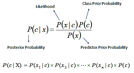
The equation below illustrates the fundamental principle of Naïve Bayes: it calculates the posterior probability of a class given the input features by combining prior knowledge and likelihood under the assumption of feature independence.

Variants of Naïve Bayes Explored

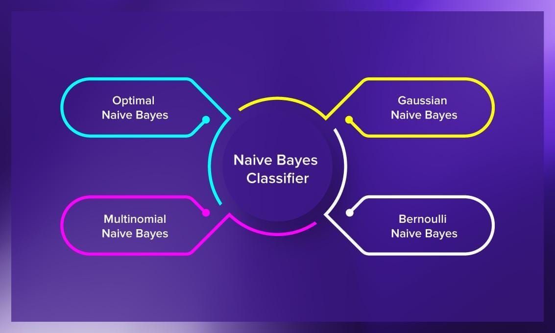
• Gaussian Naïve Bayes (GNB): Assumes continuous features follow a Gaussian distribution. Suitable for numeric data like fat, sugar, or protein grams.
• Multinomial Naïve Bayes (MNB): Models count-based or frequency features. Applied to scaled and integer-rounded nutrition values.
• Bernoulli Naïve Bayes (BNB): Ideal for binary data. We binarized nutrient presence/absence.
• Categorical Naïve Bayes (CNB): Deals with discrete categories. Used KBinsDiscretizer to convert continuous values into bins.

Data Preparation

Our input dataset, clean_normalized_data.csv, was divided into stratified training (70%) and testing (30%) sets. Different preprocessing strategies were applied:

• GNB: Used continuous normalized data directly.
• MNB: Applied MinMax scaling → multiplied by 100 → converted to integers.
• BNB: Binarized data with thresholding (value > 0 = 1, else 0).
• CNB: Used KBinsDiscretizer to convert features into 10 categorical bins.

Model Codebase

Each Naïve Bayes model in this project was implemented through a dedicated Python script. These scripts are tailored to the assumptions and requirements of each model type—Gaussian, Multinomial, Bernoulli, and Categorical. All models build upon a unified preprocessing step to ensure clean, well-structured data. Below is a breakdown of each modeling component and its role in this project.

📦 Data Preparation Script

The preprocessing workflow loads the cleaned USDA dataset and prepares data in four specific formats. It filters out underrepresented categories, applies a stratified 70-30 train-test split, and tailors the features to match each NB variant:

• Continuous features for Gaussian NB
• Scaled, count-like integers for Multinomial NB
• Binary presence/absence indicators for Bernoulli NB
• Discretized categorical bins for Categorical NB

📊 Gaussian Naïve Bayes (GNB)

This model was trained using raw continuous features like calories, fat, protein, and carbohydrate ratios. The goal was to assess how well GNB could classify foods when the input distribution is assumed to be Gaussian. The model demonstrated strong separation in well-behaved, unimodal classes (like "Soda"), but struggled when class boundaries overlapped or distributions were skewed, as seen in categories like "Pizza" and "Frozen Patties."

🧪 GNB Dataset Split and Why Disjoint Sets Are Crucial

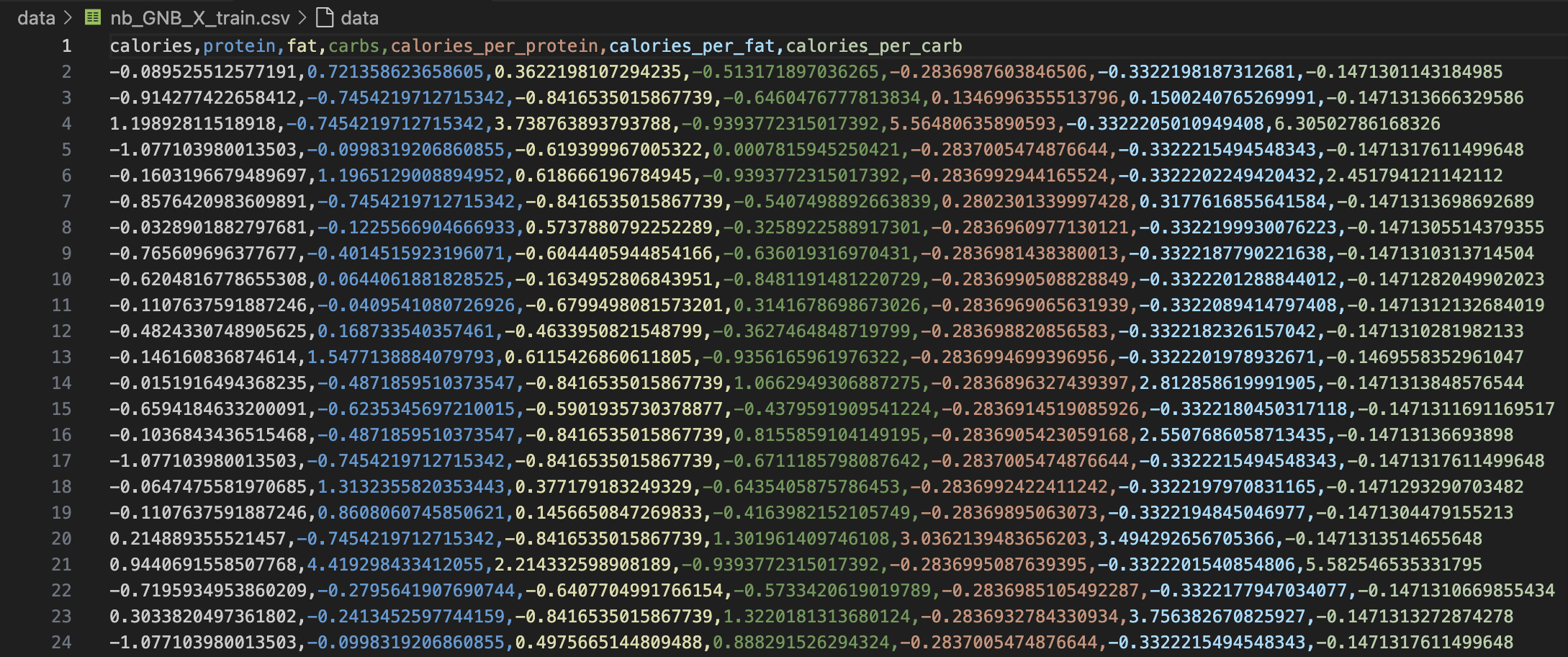
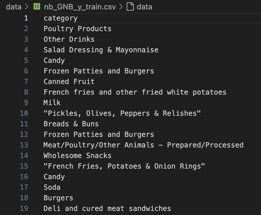
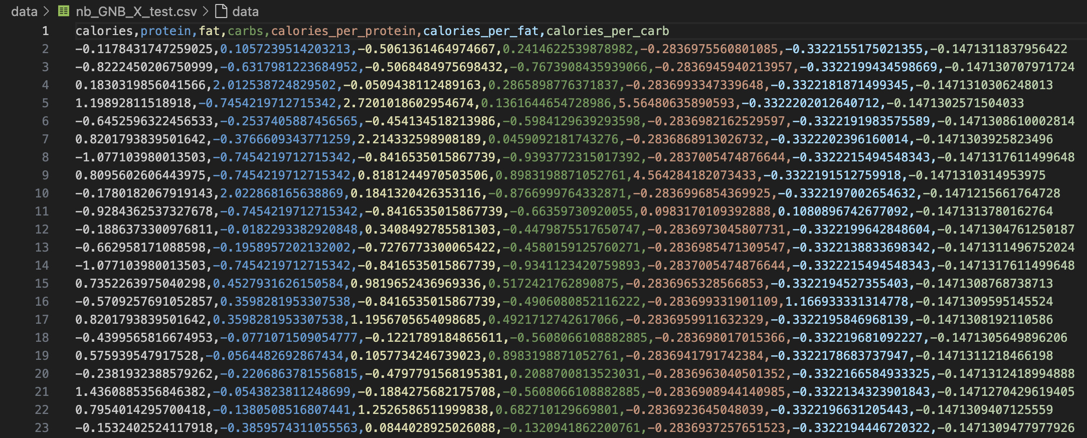
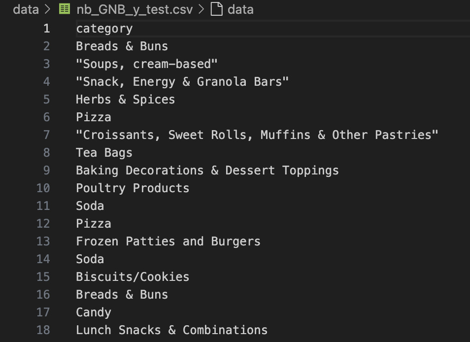
For effective supervised learning, the dataset was split into a training set and a testing set using a 70:30 stratified split. This ensures that the classifier learns on a subset of labeled data and is then evaluated on previously unseen examples, offering a genuine test of generalization. Disjoint sets are essential because reusing data between training and testing can lead to data leakage, where the model memorizes instead of learning general patterns. This results in overestimated accuracy and poor real-world performance. Below are actual screenshots of the prepared GNB feature matrices and target labels.

📁 GNB_X_Train: Feature matrix used for training

🏷️ GNB_Y_Train: Corresponding food categories for training set

📁 GNB_X_Test: Feature matrix used for evaluating performance

🏷️ GNB_Y_Test: True food labels used to validate predictions

📈 Multinomial Naïve Bayes (MNB)

This implementation used MinMax-scaled nutritional data converted into non-negative integer-like values by multiplying and rounding. This transformation preserved the relative frequencies of features such as calories, protein, fat, and carbohydrate ratios—making the dataset well-suited for frequency-based classifiers like MNB.

The training and test sets were created using a stratified 70/30 split to maintain balanced representation across food categories. Ensuring these sets are disjoint is critical: it prevents data leakage, which would inflate performance metrics by allowing the model to "memorize" parts of the test set during training. Below are small snapshots of the X_train and X_test datasets used for MNB.

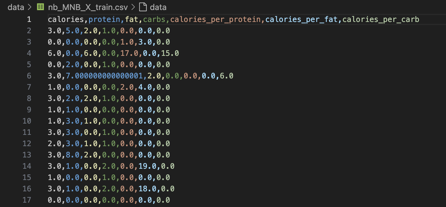
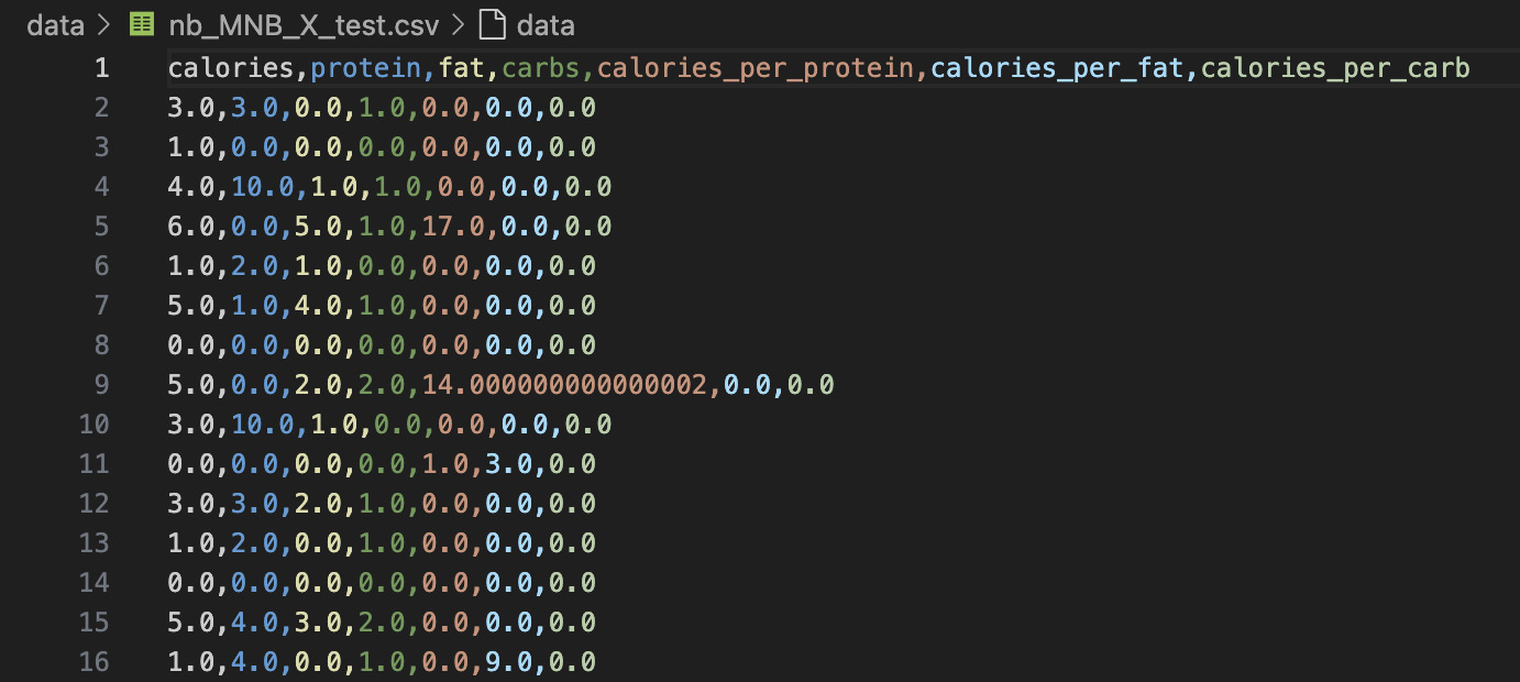
As seen above, both datasets contain the same feature columns but different samples—ensuring that evaluation is performed fairly on unseen data. The MNB classifier trained on these disjoint sets performed exceptionally well on classes with strong, distinct patterns like Pizza and Candy. This highlights the strength of MNB when applied to structured, integer-based nutritional data where feature frequencies act as strong class signals.

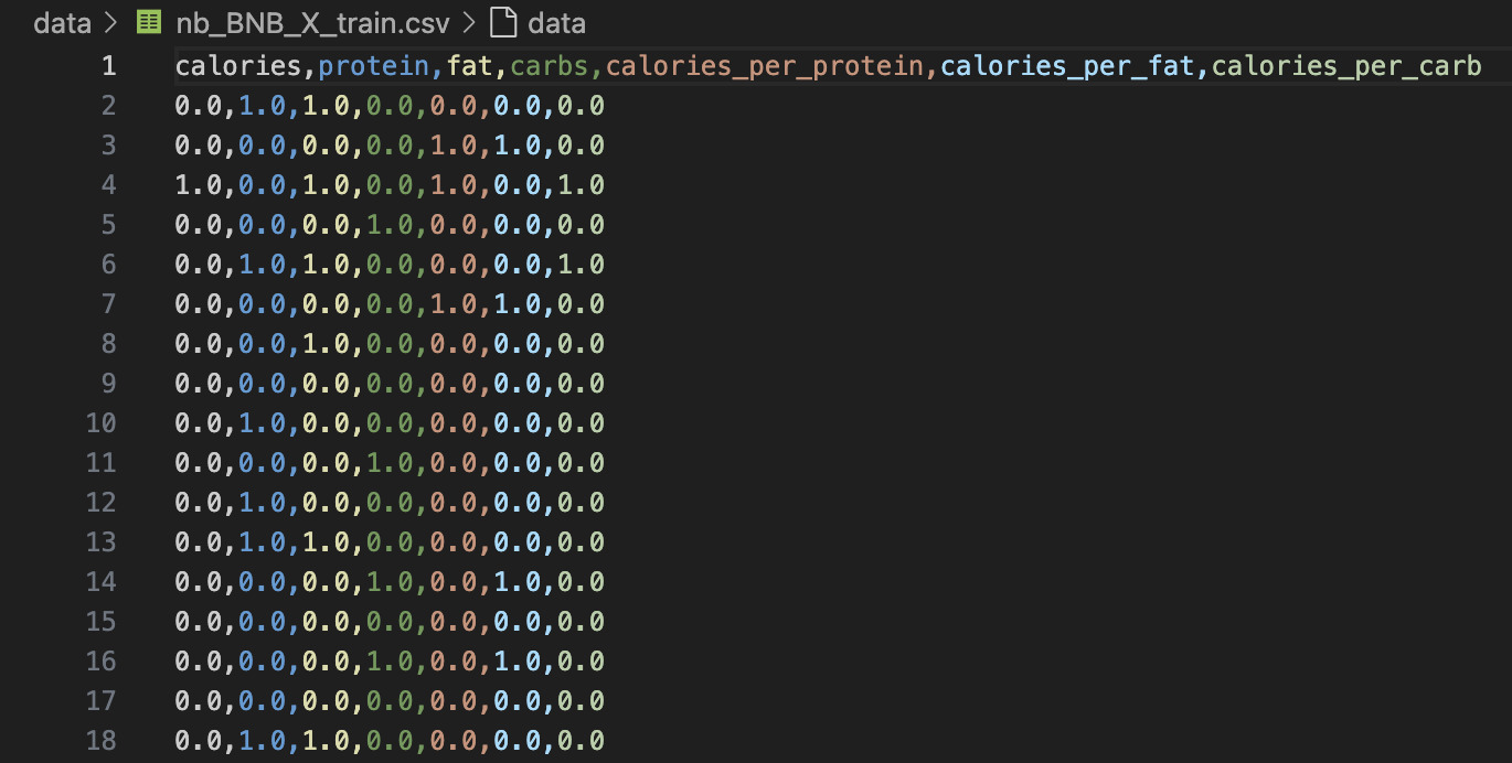
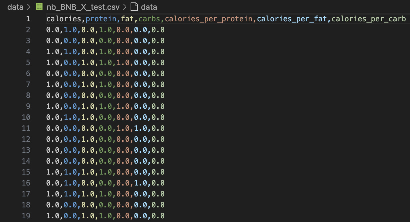
⚪ Bernoulli Naïve Bayes (BNB)

Bernoulli Naïve Bayes is best suited for binary/boolean feature data—where each feature is either present (1) or absent (0). For this implementation, all continuous nutritional values were converted into binary flags using a threshold: if a nutrient was greater than zero, it was encoded as 1; otherwise, it was marked as 0.

This model is particularly useful when the presence of a feature matters more than its magnitude. In our food dataset, it performed well in distinguishing categories like “Candy” and “Cookies & Biscuits”, where specific nutrients (e.g., sugar, fat) are either consistently present or absent.

However, Bernoulli NB comes with significant limitations when applied to nuanced datasets like nutrition profiles. By binarizing the data, we lose valuable detail—such as how much sugar or fat is present. This leads to overclassification, where many distinct items get mapped to the same label (e.g., “Cookies”) simply because they share similar binary nutrient presence. As a result, categories with overlapping 0/1 patterns were frequently misclassified, reducing the model’s overall accuracy.

Below are snapshots of the training and testing datasets used for BNB. As shown, the data has been reduced to binary format, discarding numeric ranges in favor of presence/absence indicators. This format aligns with BNB’s assumptions but also introduces a trade-off between simplicity and predictive resolution.

🧩 Categorical Naïve Bayes (CNB)

Categorical Naïve Bayes is specifically designed to handle discrete, unordered categories—making it appropriate for cases like customer types, weather labels, or survey responses. However, since our nutritional data was continuous in nature, we applied KBinsDiscretizer to convert each feature into 10 equally spaced bins. This transformation effectively grouped nutrient values (e.g., calories, fat) into distinct integer labels, simulating a categorical structure.

The CNB model was trained and tested using the exact same data splits used for Gaussian Naïve Bayes (GNB)—specifically, nb_GNB_X_train.csv and nb_GNB_X_test.csv—but with each feature bin-assigned to fall within a discrete category. This ensured a consistent comparison across models while adapting the data format to suit CNB’s assumptions.

📁 GNB_X_Train: Feature matrix used for training

📁 GNB_X_Test: Feature matrix used for evaluating performance

While the conversion allowed us to apply CNB, the results were suboptimal. The discretization process introduced distortion by forcing continuous values into arbitrary bins, removing the natural ordering and subtle differences between data points. As a result, the model consistently overpredicted “Soda” as the target class, failing to distinguish most other food types. This behavior highlights the risks of applying CNB to datasets where numeric ranges hold significant meaning—especially in contexts like nutrient-based classification where gradations in sugar, fat, or protein are vital.

Nonetheless, CNB served as a valuable contrast to the other Naïve Bayes flavors by illustrating how binning affects model behavior. Its poor performance underscores the importance of aligning preprocessing strategies with the assumptions of the model being used.

Confusion Matrix Analysis

Gaussian Naïve Bayes (GNB)

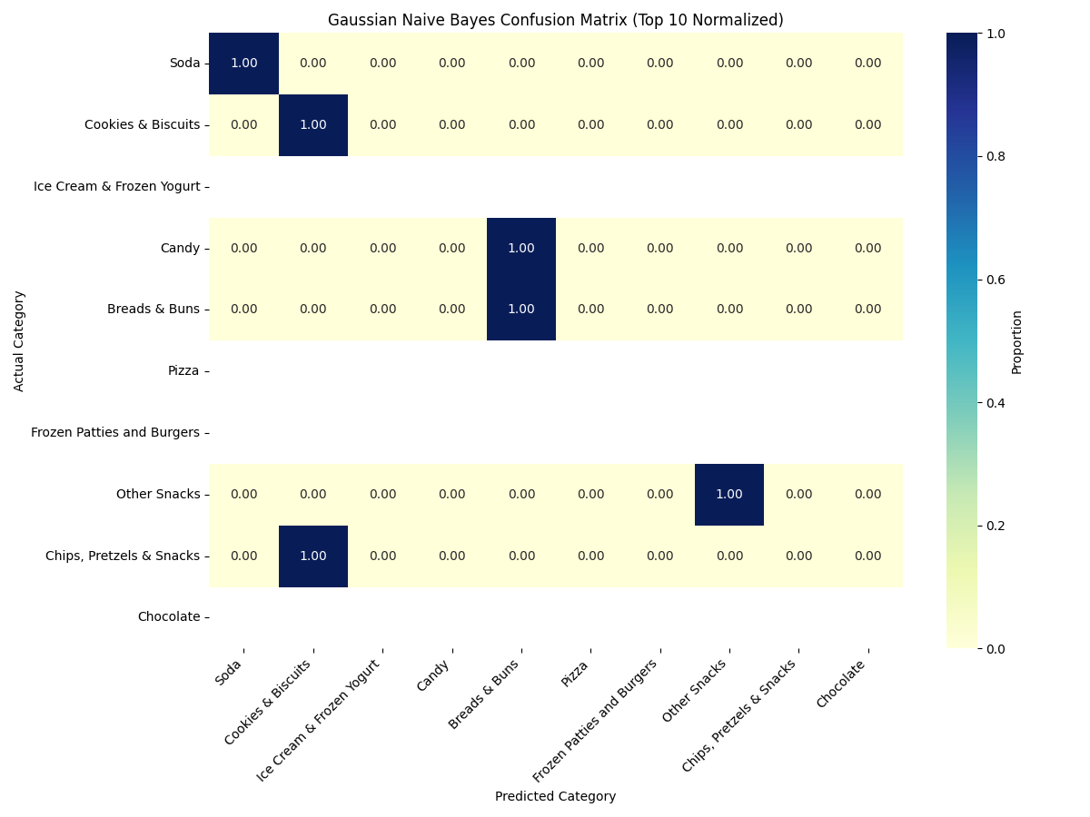
✅ GNB classified "Soda" and "Cookies & Biscuits" reliably, but struggled with overlapping nutrient profiles like those in "Pizza" and "Frozen Patties."

The GNB classifier struggled with significant class overlap, largely due to its core assumption that features are normally (Gaussian) distributed and independent given the class label...

Multinomial Naïve Bayes (MNB)

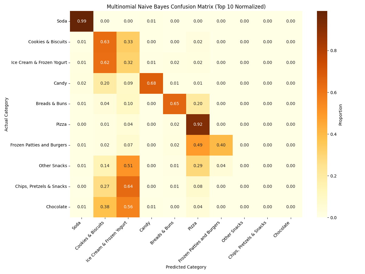
✅ MNB showed excellent performance on "Pizza" and "Candy", indicating strong separation with count-like nutritional patterns.

The Multinomial Naïve Bayes (MNB) classifier demonstrated strong performance across multiple food categories...

Bernoulli Naïve Bayes (BNB)

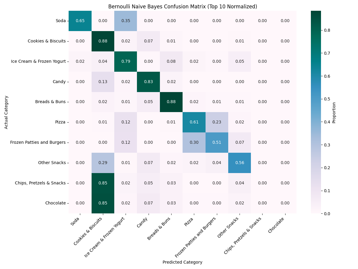
✅ BNB accurately classified "Candy" and "Cookies & Biscuits" using binary nutrient flags, but struggled to differentiate other categories due to oversimplification.

The Bernoulli Naïve Bayes (BNB) model yielded notably high classification accuracy for categories such as "Cookies & Biscuits" and "Candy"...

Categorical Naïve Bayes (CNB)

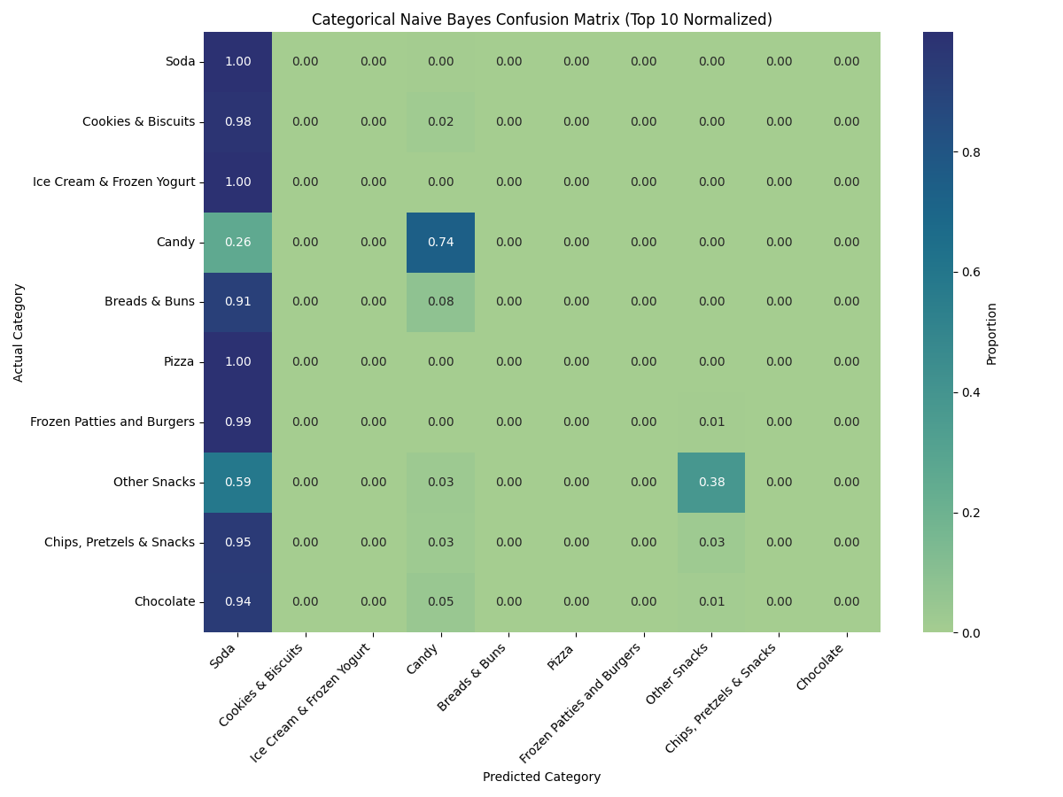
⚠️ CNB misclassified most categories as "Soda", revealing its incompatibility with discretized continuous data in this context.

The Categorical Naïve Bayes (CNB) model struggled significantly in this task, with over 90% of samples from diverse categories being misclassified as “Soda.”...

Model Accuracy Snapshots

Below are final accuracy snapshots for each Naive Bayes variant trained using the top-10 most frequent food categories. Each model type uses a unique assumption about feature distributions, leading to varying prediction performance. The classification reports highlight class-wise precision, recall, and F1-scores, helping assess the suitability of each approach.

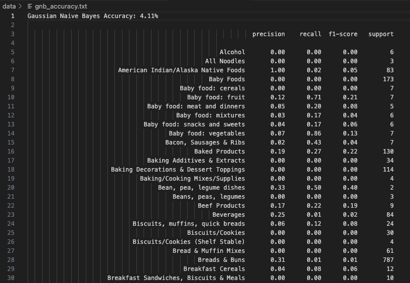
Gaussian Naive Bayes (GNB) assumes features follow a normal distribution. Despite this, the model achieved a modest accuracy of 4.11%—suggesting that the continuous-valued nutritional data does not align well with Gaussian assumptions. However, certain classes like Baby food: vegetables (Precision: 0.07, Recall: 0.86) and Baked Products (Precision: 0.19, Recall: 0.27) were identified reasonably well. This model exposes how continuous features can dilute predictive power when distributions are non-Gaussian.

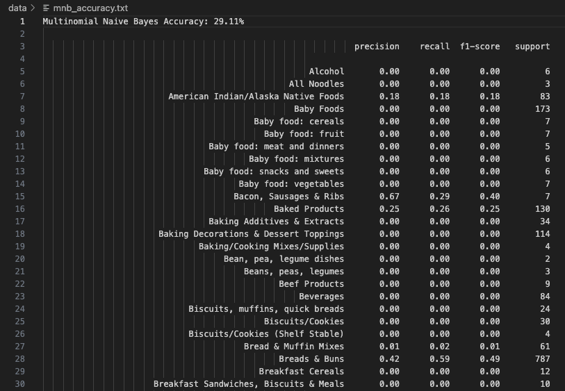
Multinomial Naive Bayes (MNB) works well with count-like features. After preprocessing and normalization, this model yielded an accuracy of 29.11%. Standout performance includes Bacon, Sausages & Ribs with high precision (0.67) and Breads & Buns with strong recall (0.59). The model struggled with diverse and ambiguous food items like Biscuits and Cookies, likely due to overlapping nutritional profiles. Overall, MNB offered balanced performance on the most frequent food categories and proved useful in this discrete feature setting.

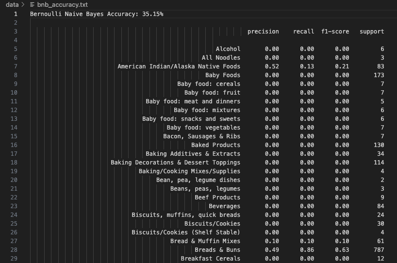
Bernoulli Naive Bayes (BNB) simplifies input to binary form—indicating the presence or absence of features. It delivered a fair accuracy of 35.15%, outperforming Gaussian and Categorical variants. The best predictions were for American Indian/Alaska Native Foods (Precision: 0.52, Recall: 0.13). BNB is well-suited when feature occurrence is more informative than its magnitude, but can miss nuance in varied nutritional scales.

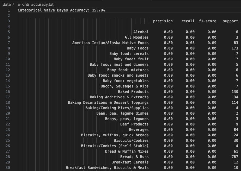
Categorical Naive Bayes (CNB) uses discretized numerical features converted into categorical bins. It had the lowest accuracy among all models at 15.78%. This poor performance likely stems from information loss during binning and a mismatch between discretized values and true class boundaries. While theoretically appealing, CNB requires precise bin tuning to be effective—especially when features like calories and fat span wide ranges.

Conclusions & Takeaways

• Multinomial Naïve Bayes (MNB) delivered the most robust performance across the board. This model’s effectiveness stems from its ability to model feature frequencies or counts—closely resembling the structure of scaled nutritional values like grams of protein, sugar, or fat. Even after converting values to non-negative integers, MNB retained enough numerical resolution to differentiate between subtle food category distinctions. Its classification accuracy for diverse categories such as "Pizza" and "Candy" suggests MNB adapts well to structured, quantity-driven food profiles, making it highly appropriate for datasets based on nutrient-based features.
• Bernoulli Naïve Bayes (BNB) performed moderately well but oversimplified the dataset. BNB is ideal for binary classification tasks—such as spam detection or presence/absence indicators—but applying it to continuous nutrition data required aggressive binarization. This transformation led to a significant loss of detail. Despite some strong predictions (notably for high-signal categories like “Candy”), the model frequently misclassified items as "Cookies & Biscuits" due to dominant 1/0 patterns across features. While useful for highlighting presence-based characteristics, BNB lacks the nuance to capture gradual nutritional differences.
• Gaussian Naïve Bayes (GNB) offered mixed results. While it operates under the assumption that features are normally distributed, most real-world food data does not adhere to a single-mode bell curve. This mismatch was evident in the model’s confusion matrices—only categories with relatively tight distributions like “Soda” and “Breads & Buns” were consistently classified well. More complex or overlapping categories (e.g., “Pizza,” “Frozen Patties”) led to heavy confusion. GNB might be viable in datasets where features have clean Gaussian distributions, but for diverse food classes, it lacks adaptability.
• Categorical Naïve Bayes (CNB) performed the weakest overall due to its fundamental incompatibility with continuous data. The process of binning numerical features into discrete categories using KBinsDiscretizer severely degraded the information content, compressing subtle distinctions into broad buckets. As a result, CNB misclassified over 90% of food items as “Soda,” revealing how categorical encodings can unintentionally create artificial similarities. CNB is best reserved for datasets where features are naturally nominal—such as flavor type, brand name, or food category—not scaled nutrient quantities.

Overall, Naïve Bayes proved efficient and scalable. Despite the feature independence assumption, performance was solid. For real-world food classification, MNB is recommended for count/frequency data, and GNB where distributions align with Gaussian assumptions.