Introduction to Decision Trees for Food Classification

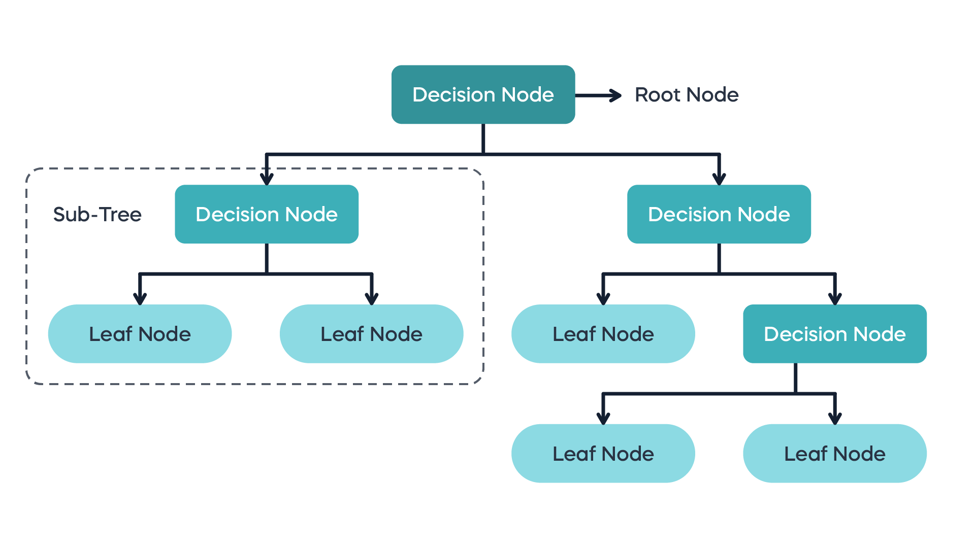
Decision Trees (DTs) are one of the most foundational and interpretable machine learning models. They operate by recursively partitioning the input data into smaller subsets based on feature values, ultimately forming a tree-like graph. Each internal node corresponds to a feature-based decision rule, each branch corresponds to the outcome of that rule, and each leaf node represents a final prediction—often a class label in classification tasks or a numerical value in regression tasks.

These models are used across a variety of domains such as medical diagnosis, fraud detection, and of course, nutritional analysis—where the relationships between features like calories, fat, sugar, and sodium can help predict food categories or healthiness levels. Decision Trees are favored because they are easy to visualize and interpret. Unlike black-box models, DTs allow us to track every decision and understand why a certain prediction was made.

However, this flexibility comes at a cost. Decision Trees are prone to overfitting, especially if allowed to grow indefinitely. This is why regularization parameters such as max_depth, min_samples_split, and min_samples_leaf are essential—they prevent the tree from memorizing the training data and failing to generalize to unseen samples.

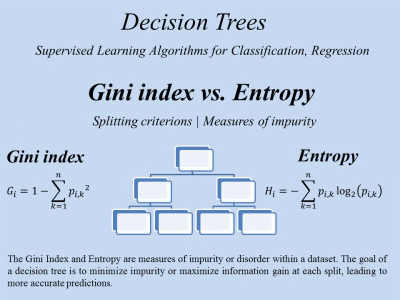
Impurity Metrics: At the core of decision tree construction lies the concept of impurity, which measures the degree of heterogeneity in a node. Two of the most popular impurity measures are:

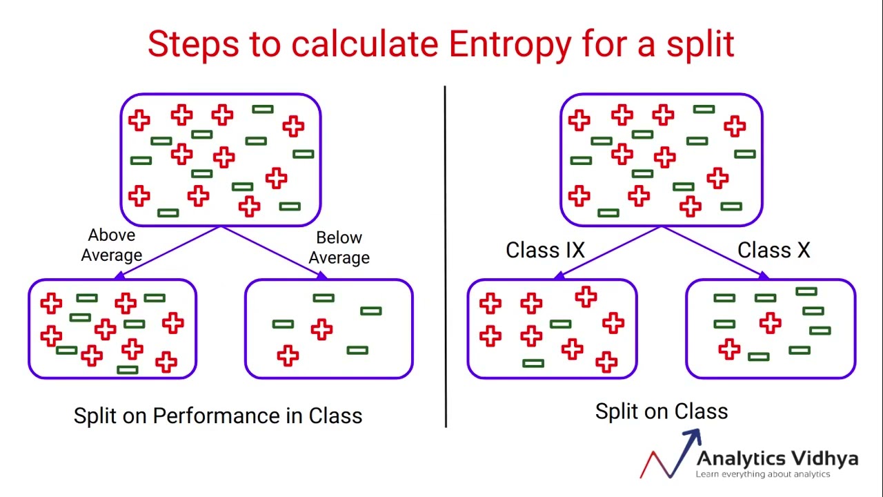
• Entropy: A concept borrowed from information theory, entropy measures the unpredictability or impurity in a dataset.
\[ H = - \sum p(x) \log_2 p(x) \]
• Gini Index: A measure of impurity that evaluates the probability of a misclassification.
\[ G = 1 - \sum p(x)^2 \]

Information Gain quantifies the effectiveness of a split by measuring the reduction in impurity. If splitting a node leads to purer subsets, that split is considered valuable. The formula is:

Illustrative Example: Consider a dataset with 10 food items: 5 are labeled as "Healthy" and 5 as "Unhealthy". The entropy at the root node is:

Now, imagine splitting based on the feature "Calories" yields two subsets: one with 4 Healthy and 1 Unhealthy (entropy = 0.72), and one with 1 Healthy and 4 Unhealthy (entropy = 0.72). Weighted average entropy of children = 0.72.

This means the split reduced impurity and added predictive power.

It's also important to understand that Decision Trees can grow indefinitely. At every level, the algorithm tries to further split the data to gain slightly more information. If unchecked, it could result in a tree with one leaf per training example. This is known as overfitting. To avoid it, tree growth is constrained using pruning or limiting parameters like max_depth. Thus, although infinite trees are possible, they’re rarely desirable.

In food classification tasks, Decision Trees serve as a powerful baseline because they reflect intuitive patterns in nutrition. For example, high sugar and low protein might signal Candy or Soda, while moderate calories and high fat could point to Pizza or Burgers. These models allow for both interpretability and feature-based hypothesis generation, making them a valuable tool in exploratory and predictive food analysis.

Data Preparation

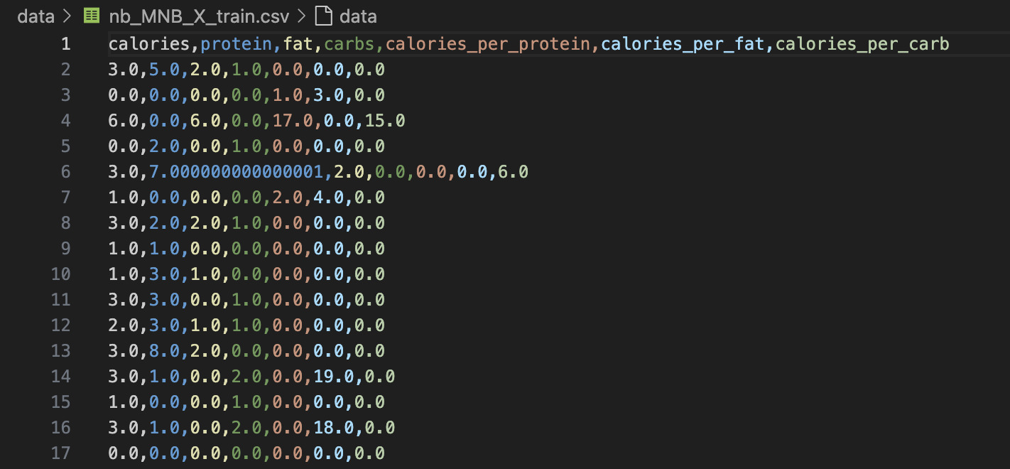
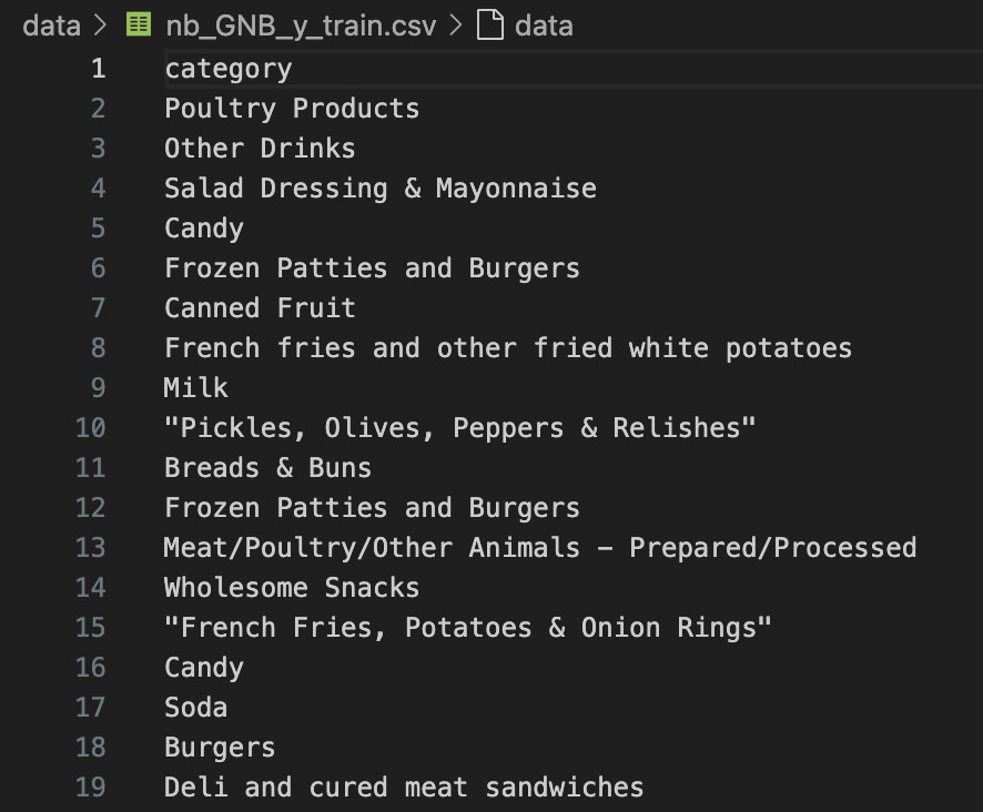
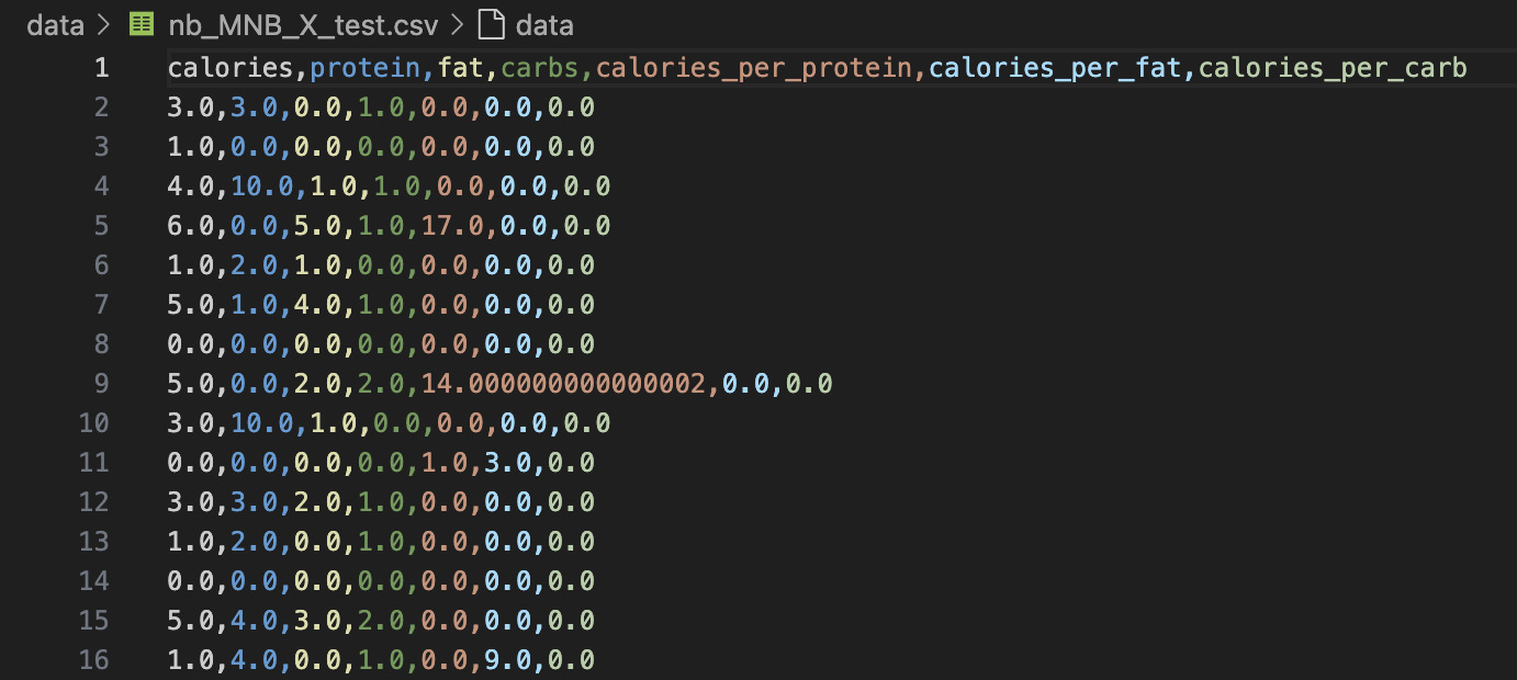
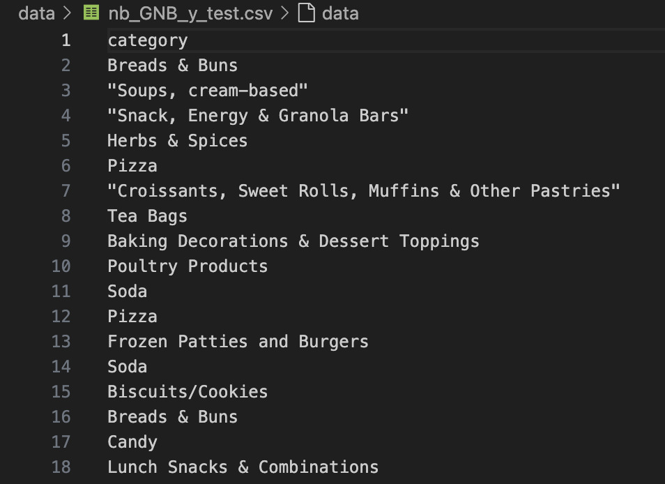
We used the same cleaned and preprocessed nutritional dataset from Multinomial Naïve Bayes for consistency. The feature matrices were taken from nb_MNB_X_train.csv and nb_MNB_X_test.csv, while the corresponding labels were pulled from nb_GNB_y_train.csv and nb_GNB_y_test.csv.

A 70:30 stratified train-test split was applied to maintain proportional class distribution across both sets. Ensuring these sets are disjoint is critical to avoid data leakage—where knowledge of the test set contaminates the training process, leading to inflated accuracy and poor real-world generalization.

📁 X_train: Feature matrix for training

🏷️ y_train: Labels for training

📁 X_test: Feature matrix for evaluation

🏷️ y_test: Ground truth labels for evaluation

Model Codebase

The Decision Tree models were implemented using Scikit-learn’s DecisionTreeClassifier. Three separate trees were trained using different root nodes by customizing max_features or manually selecting feature importance to control splitting. Evaluation was performed on the test set.

Results and Visualizations

This section presents classification results using multiple variants of the Decision Tree model. The analysis explores how different nutrient-related root splits—namely calories, protein, and fat—impact the prediction of food categories. A normalized confusion matrix and accuracy visuals are also included to support the model evaluation.

Normalized Confusion Matrix

The matrix below shows the model’s performance on the top-10 most active food categories. Rows represent the true labels and columns the predicted ones. By normalizing values, we can better compare performance across classes.

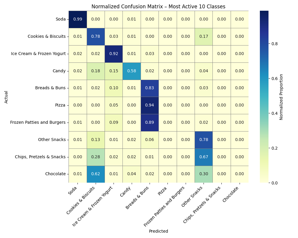
The model demonstrates strong accuracy for categories like Soda, Pizza, and Ice Cream & Frozen Yogurt, with over 90% correct predictions. However, overlapping nutrient profiles lead to confusion between Cookies & Biscuits, Chocolate, and Chips & Pretzels. These confusions suggest a need for finer-grained features or ensemble methods in future modeling.

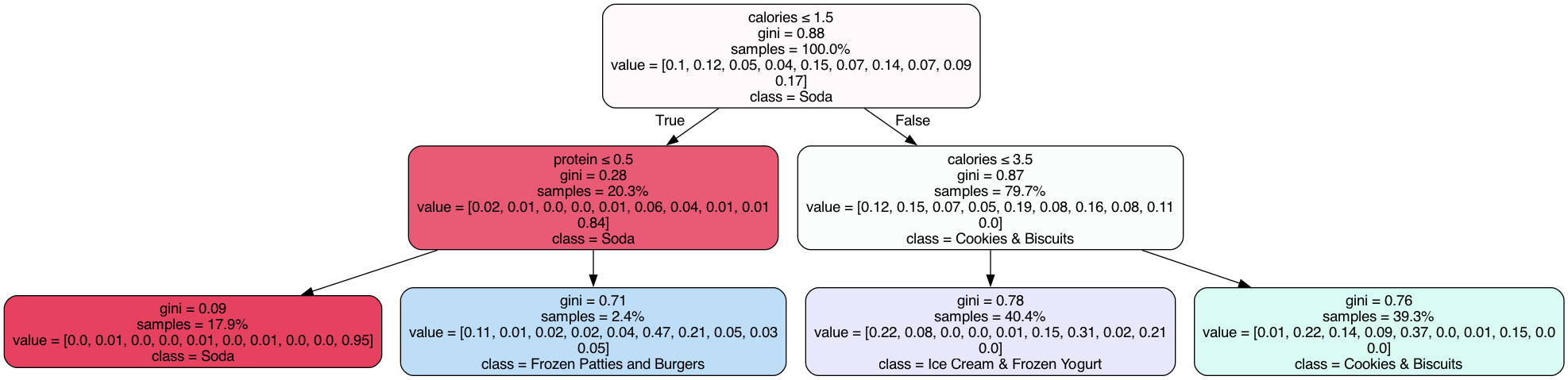
Tree Variant 1 – Root: calories

The first decision tree variant uses calories as its root feature. It divides the data into low- and high-calorie items, leading to a dominant first split for Soda. Subsequent branches focus on protein to separate categories like Frozen Patties & Burgers and Ice Cream. This tree is the most balanced in terms of generalization and interpretability.

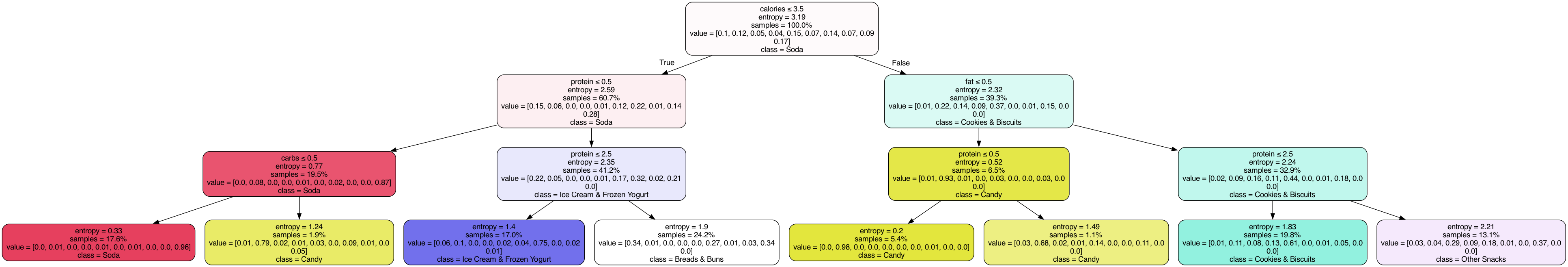
Tree Variant 2 – Root: protein

This variant begins with protein as the root node, isolating high-protein and low-protein foods early. Notably, Candy and Soda are separated efficiently at shallow depths due to their distinct low-protein content. However, this tree becomes more complex in mid-level branches and may be prone to misclassifying high-carb desserts such as Cookies and Chocolate.

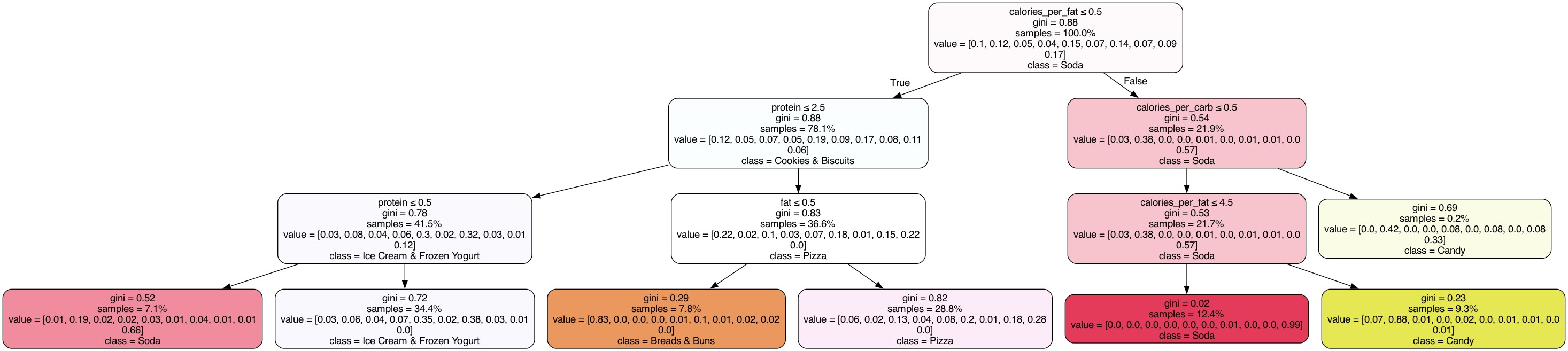
Tree Variant 3 – Root: fat

The third variant explores fat as the root splitting criterion. This leads to early separation of Breads & Buns and Cookies & Biscuits. Although visually deeper, the tree reveals clearer clustering for Pizza and Candy in later splits. This variant offers a unique view into how fat-related nutrient structure contributes to classification.

Model Accuracy Snapshots

Below are final accuracy snapshots for each Decision Tree variant trained using the top-10 most frequent categories in the dataset. Each model varies in terms of its splitting strategy or root feature selection. The classification reports highlight class-wise precision, recall, and F1-scores.

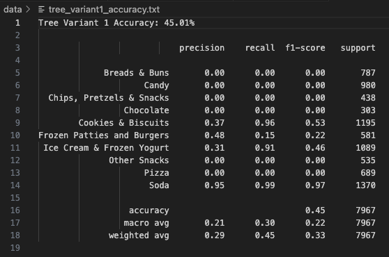
Tree Variant 1 employed a Gini-based criterion with a shallow depth and fewer splits, making it the simplest of the three trees. This model achieved an overall accuracy of 45.01%, with outstanding performance in identifying Soda (Precision: 0.95, Recall: 0.99) and Cookies & Biscuits. However, categories like Pizza, Chips, Pretzels & Snacks, and Chocolate had extremely poor recall and were often misclassified. This model seems to favor high-frequency, high-contrast categories while ignoring those with ambiguous features. The macro average F1-score is just 0.22, reflecting low generalizability. Despite its simplicity, this model shows how tree-based models can struggle when class imbalance and feature similarity are high. Tree Variant 1 is good for interpretability but not optimal for high accuracy. It demonstrates how a dominant class like Soda can influence decision boundaries disproportionately.

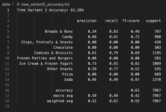
Tree Variant 2 uses entropy as the splitting criterion, along with a slightly deeper structure and stricter leaf size conditions. This change led to a significant boost in performance, achieving 62.26% overall accuracy. Categories like Candy, Ice Cream & Frozen Yogurt, Cookies & Biscuits, and Soda were predicted well. Precision for Candy was 0.88 and recall was 0.61, indicating a reliable but not perfect boundary. However, Pizza and Chips, Pretzels & Snacks still faced misclassification issues. The macro average F1-score increased to 0.42, and the weighted average reached 0.55, showing improved model stability. This variant shows the value of entropy-based information gain in dealing with class overlap. It balances performance across more classes than Variant 1, making it a better fit for datasets with moderate complexity.

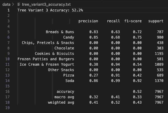
Tree Variant 3 incorporates feature restriction (max_features=2) to increase diversity and prevent overfitting. It achieved a respectable 52.20% accuracy, better than the Gini-based variant but lower than the entropy model. Notably, Breads & Buns had high precision (0.83) and recall (0.63), and Candy also performed well (Precision: 0.85, Recall: 0.68). The model struggled with Cookies & Biscuits, showing 0 values across all metrics — likely due to being overshadowed by similar categories. This variant also improves generalizability while sacrificing some recall for minority classes. The macro F1-score stood at 0.36, and the weighted F1 was 0.43. It’s a great example of how controlled randomness in feature selection can reduce overfitting but needs fine-tuning for nuanced classes. Tree Variant 3 gives an alternative look into how diversity in decision paths impacts model outcomes.

Conclusions & Takeaways

• Decision Trees provide clear interpretability and are easy to implement on structured datasets like food nutrition.
• Entropy and Gini both worked well, but Entropy-based splits yielded higher Information Gain for our dataset.
• Tree depth control is vital; unregulated trees tend to overfit. Simpler, pruned trees had better generalization.
• Root node selection significantly influenced classification accuracy, with "Calories" and "Fat" yielding the most distinct branches.

Overall, Decision Tree modeling helped uncover key nutrient features that contribute most to food category classification, offering both prediction capability and nutritional insight.