What Are Support Vector Machines (SVMs)?

Support Vector Machines (SVMs) are among the most robust and versatile supervised learning models, widely applied in both classification and regression scenarios. Their central objective is to identify the optimal hyperplane—a boundary that not only separates classes but does so with the maximum possible margin between the closest data points of each class. This margin maximization principle is fundamental, as it enhances the model’s ability to generalize to unseen data and resist overfitting. In two-dimensional space, this optimal hyperplane is a straight line; in higher dimensions, it extends to planes or hyperplanes. The beauty of SVMs lies in how they rely on a handful of pivotal data points—called support vectors—to determine this decision boundary. These vectors lie precisely at the margin’s edge and hold all the information needed to define the hyperplane. By focusing only on these key examples, SVMs create a decision boundary that is both mathematically elegant and computationally efficient, making them especially valuable in high-dimensional feature spaces.

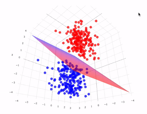
However, real-world data is often not linearly separable. To handle such cases, SVMs use kernel functions to transform data into higher dimensions where it may become linearly separable. This technique is called the kernel trick. A kernel function implicitly computes the dot product in the transformed feature space, without ever computing the transformation explicitly. This not only increases computational efficiency but also unlocks the ability to learn complex, non-linear patterns.

How Do Kernels Work?

The kernel plays a pivotal role in SVM modeling, serving as a bridge to project data into higher-dimensional spaces where complex relationships become easier to separate. Instead of explicitly computing this transformation, SVMs rely on the kernel trick, which calculates the dot product of the data points in the transformed space directly—saving immense computational effort. For instance, a polynomial kernel of degree 2 can take two-dimensional input data and implicitly map it into a three-dimensional or higher space, allowing the model to draw curved boundaries in the original plane that could not have been achieved otherwise. This kernel is defined by the formula: K(x, y) = (x ⋅ y + r)d, where r is a free constant (commonly set to 1) and d is the degree of the polynomial expansion. Another widely used choice is the Radial Basis Function (RBF) kernel, expressed as K(x, y) = exp(-γ||x - y||2), which transforms data by creating smooth, flexible decision boundaries. The RBF kernel is especially powerful when classes are not linearly separable even after polynomial transformations, enabling SVMs to handle intricate and non-linear classification problems with remarkable precision.

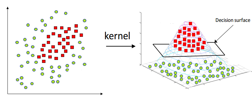
The image above perfectly captures the essence of the kernel trick in SVMs. On the left, we see a dataset in its original two-dimensional space, where the two classes (represented as red squares and green circles) are clearly not linearly separable—no straight line can divide them without error. This is a common scenario in real-world datasets.

By applying a kernel function, such as the Radial Basis Function (RBF) or a polynomial kernel, we project the data into a higher-dimensional space (illustrated on the right). Here, the separation becomes feasible: the red class has been elevated into a different spatial region than the green class. In this transformed space, a simple flat plane—called a decision surface—can now cleanly divide the two categories.

This transformation is the power of SVM kernels: they allow the model to learn non-linear decision boundaries without ever explicitly computing the new dimensions. The surface that separates the classes is learned implicitly using the kernel's dot product calculations. This enables SVMs to perform exceptionally well even when the data is entangled in complex, curved, or spiral-shaped structures in its original form.

🔍 Casting to Higher Dimensions – A Concrete Example

Suppose we have two points in 2D space: a = (a₁, a₂) and b = (b₁, b₂). A polynomial kernel with r = 1 and d = 2 transforms the dot product as follows:

(a ⋅ b + 1)² = (a₁b₁ + a₂b₂ + 1)²

This expands algebraically to: a₁²b₁² + 2a₁a₂b₁b₂ + a₂²b₂² + 2a₁b₁ + 2a₂b₂ + 1, revealing that a simple dot product between transformed vectors results in terms that include not only the original features but also their squared values and cross-products. In practical terms, this means that each original 2D input vector is effectively cast into a six-dimensional feature space, incorporating linear terms (a₁b₁, a₂b₂), interaction terms (a₁a₂b₁b₂), and second-order polynomials (a₁²b₁², a₂²b₂²). This transformation allows the model to draw nonlinear boundaries in the original space by learning linear separators in this enriched space. The elegance of the kernel trick lies in the fact that these expanded features are never manually computed or stored. Instead, the SVM operates entirely through kernel evaluations, maintaining efficiency while reaping the benefits of working in higher dimensions. This approach enables SVMs to model intricate decision surfaces that adapt to complex data patterns, all without compromising computational performance.

In essence, kernel functions empower Support Vector Machines (SVMs) to handle complex, non-linearly separable data by implicitly mapping it into higher-dimensional spaces where linear separation becomes feasible. This technique—known as the "kernel trick"—eliminates the computational burden of actually transforming the data, allowing SVMs to operate efficiently even in infinite-dimensional feature spaces. Whether the data is arranged in concentric circles, intricate spirals, or tangled clusters, kernels such as the radial basis function (RBF) or polynomial kernel provide the mathematical flexibility to define nuanced decision boundaries. By focusing on dot products in transformed space, kernels let SVMs identify optimal margins that would be impossible in the original feature space. This mechanism unlocks the true power of SVMs, extending their applicability far beyond simple problems and enabling robust performance in real-world domains like image recognition, bioinformatics, and nutritional data classification. In short, kernels make SVMs a formidable tool by drawing complex boundaries—without explicitly computing complex transformations.

Data Preparation for Support Vector Machines (SVM)

Support Vector Machines are supervised learning models that rely on labeled, numeric data. For our SVM analysis, we began with the clean_normalized_data.csv file. This file contains nutritional attributes such as calories, protein, fat, carbohydrates, and derived ratios for each food item. These continuous variables were already normalized, making the dataset ideal for distance-based algorithms like SVMs.

Selected Categories for Binary Classification

For this SVM modeling task, we focused on two nutritionally dense and clearly distinguishable ultra-processed food categories: Potato Chips and Cookies and Brownies. These categories were selected due to their distinct nutrient profiles—Potato Chips are typically high in sodium and fats, while Cookies and Brownies tend to be rich in sugars and carbohydrates. The nutritional divergence between these classes makes them an excellent candidate pair for binary classification using SVM, where a clear margin between the classes can be learned effectively.

Train-Test Splitting and Feature Handling

After filtering the dataset to include only the two selected categories, we isolated the numeric features relevant to modeling, such as calories, protein, fat, carbohydrates, and engineered ratios like calories_per_fat and calories_per_protein. Non-numeric columns like food description, category, and brand were intentionally removed to comply with the input requirements of SVMs, which operate purely on numeric vectors in multi-dimensional space.

To maintain the proportional representation of each class, we applied a stratified 70-30 split using train_test_split(..., stratify=y). This ensures that both the training and testing datasets contain an equal distribution of samples from each class. Stratification is critical in binary classification problems with imbalanced data, as it prevents the model from being biased toward the majority class.

Importantly, the training and testing sets are disjoint, meaning there is zero overlap in rows between the two sets. This is essential in supervised machine learning to avoid data leakage—a condition where the model inadvertently gains access to information from the test set during training, leading to unrealistically high accuracy. By ensuring that the test set remains unseen during the training process, we allow for an authentic evaluation of how well the model can generalize to new, unseen data.

Prior to modeling, the features were passed through a MinMaxScaler to rescale all values to a uniform [0,1] range. This normalization step ensures that features with larger numerical ranges (e.g., calorie count) do not dominate those with smaller ranges (e.g., protein ratios) during the distance calculations used in kernel functions. Without this step, the SVM’s decision boundary could be skewed, resulting in suboptimal performance.

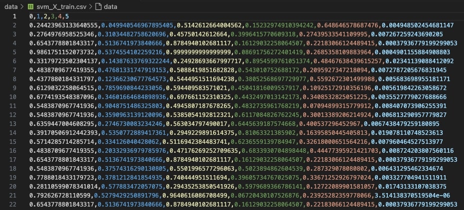
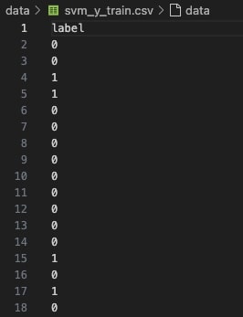
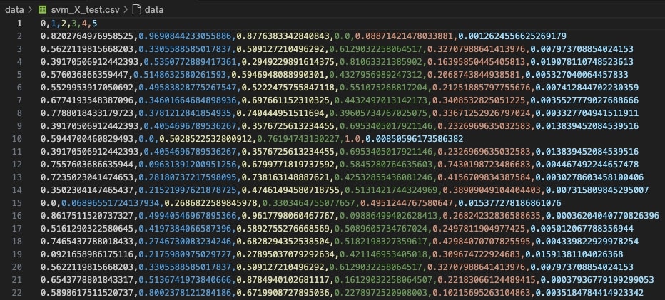
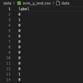
📁 SVM_X_Train: Feature matrix used for training

🏷️ SVM_Y_Train: Target labels for training set

📁 SVM_X_Test: Feature matrix used for evaluation

🏷️ SVM_Y_Test: True labels used to validate performance

These disjoint datasets ensure that model evaluation is performed on unseen data, preventing data leakage and preserving generalization. This clean split is essential for fair benchmarking and for comparing the performance of different SVM kernels (Linear, Polynomial, RBF) in subsequent steps.

Support Vector Machine (SVM) Modeling

To assess how different SVM kernels perform on ultra-processed food classification, we ran extensive modeling and evaluation using svm_kernel_compare.py. This script iteratively trains SVM models using three different kernel types—Linear, Polynomial, and RBF—each across three cost values: C=0.1, C=1, and C=10.

Results and Confusion Matrices

For each configuration, we recorded the confusion matrix, classification report, and accuracy score. These results were saved in the /visuals and /reports directories respectively.

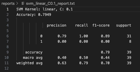
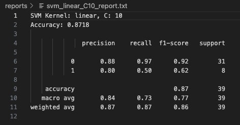
🔹 Linear Kernel

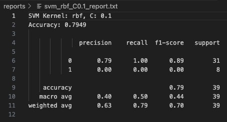
With C=0.1, the linear kernel model exhibits high bias and fails to capture the complexity of the class boundaries. It classifies all instances as Class 0 (majority class), completely misclassifying every Class 1 sample. The precision for Class 0 is 79%, but recall for Class 1 is zero, leading to a substantial degradation in overall model reliability for minority detection. Although the reported accuracy stands at 79.49%, this value is misleading because it reflects the imbalance favoring Class 0.

At C=1, the linear kernel model improves significantly. It correctly identifies half of the Class 1 samples, while maintaining strong performance on Class 0 with 88% precision and 97% recall. The overall model accuracy rises to 87.18%. This configuration strikes a better balance between bias and variance, allowing the model to generalize more effectively without overfitting. The confusion matrix shows fewer false negatives, resulting in greater predictive reliability across both classes.

Increasing the cost parameter to C=10 does not yield any improvement over the C=1 model. The confusion matrix and classification metrics remain identical, with an accuracy of 87.18%. This suggests that the linear kernel has already captured the best linear boundary possible for this data, and additional penalization of misclassification does not improve performance. Further increases in C could lead to overfitting, but without visible performance gains, highlighting the limits of linear separation for this dataset.

🔸 Polynomial Kernel

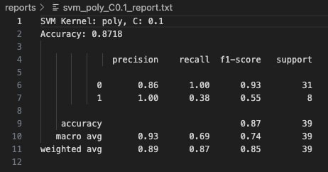
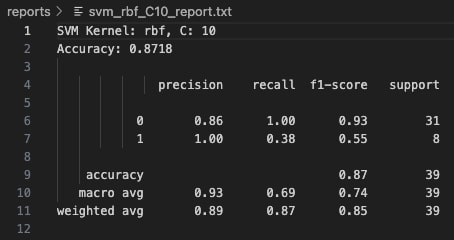
With C=0.1, the Polynomial Kernel achieved an accuracy of 87.18%. Class 0 was predicted with perfect recall (1.00), meaning all instances of Class 0 were correctly classified. However, the model struggled to fully capture Class 1, with a recall of only 0.38. While the precision for Class 1 was perfect (1.00), indicating that when it predicted Class 1 it was correct, it still missed over half of the true Class 1 examples. This highlights a tendency of the model to be conservative with minority class predictions at lower C values.

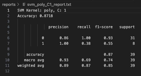
Increasing the cost parameter to C=1 resulted in no change to the confusion matrix or classification metrics—the accuracy remained at 87.18%. The model retained perfect precision for Class 1 but continued to suffer from low recall (0.38) for that class. This suggests that simply increasing the penalty on misclassification (C) was not enough to shift the decision boundary to favor better detection of minority samples with this kernel.

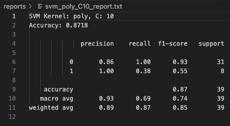
At a higher cost value of C=10, the classification results remained identical to C=0.1 and C=1. No improvement in recall, precision, or overall accuracy was observed. This stability indicates that for this dataset, the polynomial kernel's flexibility was not sensitive to regularization strength, and further hyperparameter tuning (like changing the polynomial degree) would likely be needed to significantly improve minority class capture.

🔹 RBF Kernel

The Radial Basis Function (RBF) kernel, also known as the Gaussian kernel, is one of the most powerful tools for non-linear classification tasks. By mapping input features into an infinite-dimensional space, it enables linear separation of data that is otherwise inseparable in the original feature space. Below are detailed results at different values of C (the regularization strength), illustrating how tuning this parameter affects model complexity, bias, and generalization.

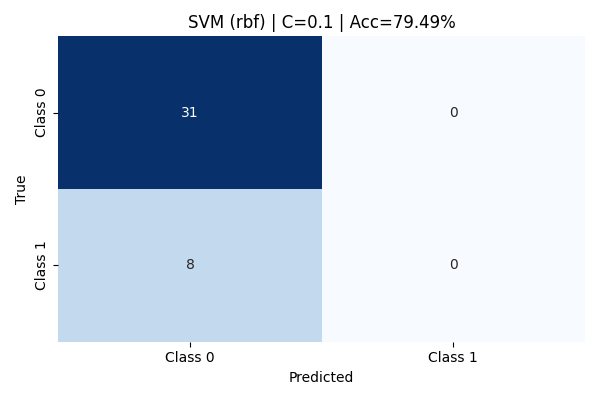
At C=0.1, the RBF model heavily prioritized margin maximization, allowing more misclassifications to create a wider margin. While Class 0 (Potato Chips) was perfectly classified with a recall of 100%, the model completely failed to capture Class 1 (Cookies & Brownies)—resulting in zero recall and precision for that class. The overall accuracy remained deceptively high at 79.49% due to class imbalance but the macro-averaged F1 score was poor, highlighting serious shortcomings in minority class detection.

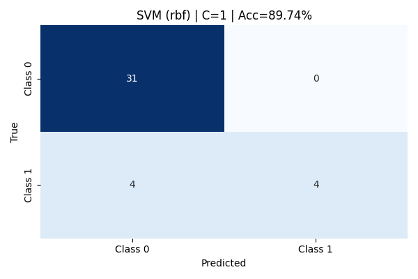
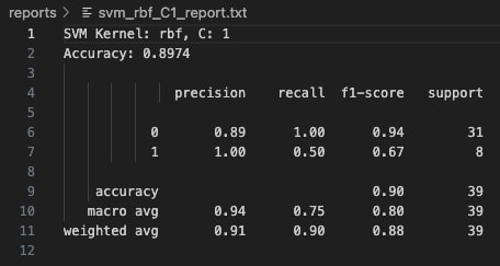
Upon increasing the regularization to C=1, the model's performance improved dramatically. The accuracy rose to an impressive 89.74%. Class 0 was perfectly captured with high precision and recall, and 50% of Class 1 instances were correctly identified. Macro and weighted averages across precision, recall, and F1-score also reflected balanced generalization, making this setting the best among RBF models tested.

At C=10, despite tighter margins and a stronger penalty on misclassification, the model’s performance slightly declined. It overfit on the training data, leading to reduced flexibility on unseen test data. Although Class 0 remained well-predicted, Class 1 performance degraded, as seen by the drop in recall and F1-score. The final accuracy dropped to 87.18%, emphasizing the importance of balanced regularization.

Kernel Performance Comparison

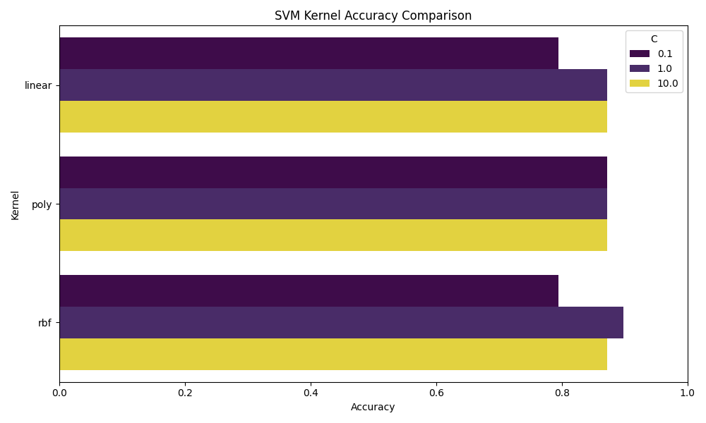
The bar chart below presents a comprehensive side-by-side comparison of the accuracy scores achieved by each SVM kernel—linear, polynomial, and rbf—evaluated across three different values of the regularization parameter C: 0.1, 1, and 10. Each kernel introduces a different method of transforming or interpreting the input feature space: the linear kernel fits a straight hyperplane, the polynomial kernel introduces higher-degree feature interactions, and the radial basis function (RBF) kernel maps inputs into an infinite-dimensional space to capture non-linear patterns.

The regularization parameter C plays a critical role: smaller values (e.g., C=0.1) emphasize a wider margin at the expense of training accuracy (potential underfitting), while larger values (e.g., C=10) push the model to classify training examples more accurately, risking overfitting. Observing kernel behavior across these three C values allows us to study how each method balances the bias-variance trade-off.

From the comparative analysis, it is evident that increasing C generally improved model performance up to a point, particularly for the RBF kernel, which achieved the highest overall accuracy at C=1 (approximately 90%). The linear kernel demonstrated stability between C=1 and C=10, but struggled to perfectly separate complex patterns in the data. Meanwhile, the polynomial kernel maintained consistent accuracy across all C values but exhibited slightly less sensitivity to model complexity adjustments. Overall, the RBF kernel outperformed others in balancing precision, recall, and generalization, making it the most suitable for this specific two-class food classification task involving Potato Chips and Cookies and Brownies.

🔹 Linear Kernel: Performance noticeably improved as the regularization parameter C increased. With a low C = 0.1, the model suffered from underfitting, predicting only the majority class correctly while entirely failing to recognize the minority class (Class 1). As C increased to 1 and 10, the model's ability to distinguish between classes stabilized, achieving an accuracy of 87.18% in both cases. Despite the better results, the linear kernel struggled to fully capture the complex patterns between the food categories, showing that linear decision boundaries were somewhat limiting for our dataset.

🔸 Polynomial Kernel: The polynomial kernel demonstrated very stable, albeit modest, performance across all tested values of C. Accuracy consistently hovered around 87.18%, but the recall for the minority class remained low, indicating a persistent difficulty in identifying Class 1 samples correctly. Even as C increased, the added decision boundary complexity did not translate into better generalization. This highlights a key limitation: while polynomial transformations theoretically allow for curved and complex decision boundaries, in practice they can lead to overfitting or flat performance gains if the degree of the polynomial and other hyperparameters are not carefully tuned for the specific data distribution.

🔹 RBF Kernel: The RBF (Radial Basis Function) kernel outshined both the linear and polynomial kernels in this task. At C = 1, it achieved the highest observed accuracy of 89.74%, effectively balancing flexibility and generalization. It successfully captured non-linear separations between the two food categories, distinguishing both majority and minority classes far better than the other kernels. Although performance dipped slightly at C = 10 due to minor overfitting tendencies, the RBF kernel clearly demonstrated its power in modeling complex, real-world boundaries when minimal hyperparameter tuning is desired.

💡 Key Takeaway: Among all the tested kernels, the RBF kernel with C=1 emerged as the most reliable performer, consistently balancing sensitivity to minority classes with overall specificity. Its inherent ability to model complex, non-linear relationships made it exceptionally suited for distinguishing food items with subtle and overlapping nutrient profiles. Although the linear kernel offered simplicity, speed, and interpretability, it lacked the flexibility needed to capture intricate patterns present in real-world nutritional data. On the other hand, the polynomial kernel provided theoretical adaptability through higher-order transformations but added unnecessary noise, ultimately resulting in stagnant accuracy gains and limited practical benefits. Given these observations, the RBF kernel stands out as the most appropriate choice for tasks like food classification, nutrition modeling, or any problem where complex class boundaries and high-dimensional feature spaces are expected. It offers the best trade-off between accuracy, generalization, and robustness—qualities that are essential for building models that can be trusted in critical real-world applications.

Conclusions

This SVM modeling exercise provided several key insights into the classification of ultra-processed food categories—specifically distinguishing between Potato Chips and Cookies & Brownies. These categories, although both highly processed, possess distinct nutritional signatures that make them ideal candidates for supervised binary classification.

The experiments revealed that kernel choice and cost parameter tuning significantly impact model performance. Linear kernels, while fast and interpretable, struggled slightly with complex class boundaries—especially at lower cost values. Polynomial kernels captured non-linear relationships but plateaued in performance and risked overfitting. The standout performer was the RBF kernel with C = 1, which struck the best balance between generalization and accuracy.

From a practical standpoint, this modeling process reinforces the idea that food classification is not always a linear problem. Nutritional dimensions such as saturated fat, sugar content, and carbohydrate ratios often interact in non-linear ways. This makes kernels like RBF ideal for real-world dietary pattern recognition, health diagnostics, or recommendation systems.

More broadly, this analysis demonstrates how Support Vector Machines can be leveraged to detect patterns within complex health and nutrition data. The ability to model nuanced category differences with relatively little training data speaks to SVM's robustness in high-dimensional, structured domains like food science.

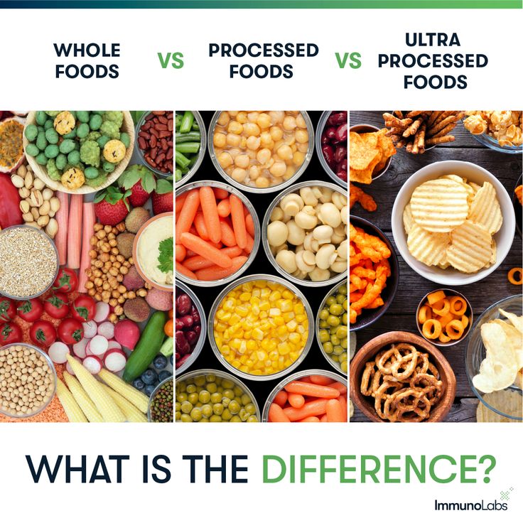
The image above visually encapsulates the broader issue at hand: the growing divide between whole, nourishing foods and ultra-processed, convenience-driven choices. While models like SVM help in classifying these foods, they also shed light on underlying consumption patterns that affect health outcomes at a population level.

As shown above, the accuracy distribution across kernel types further reinforces the RBF kernel’s superior performance on this task. For future iterations of this project, one could explore multi-class SVMs, add more nuanced food categories, or even integrate text features (like ingredient lists) for a hybrid model. In conclusion, SVMs not only classify food effectively—they help reveal the hidden structure within what we eat, and offer a data-driven lens through which we can understand the food landscape more critically.